
Cortex-A & Cortex-M - Qeexo's Custom Virtual Sensor Board
.png?inst-v=0e115e88-76f5-42af-928f-0447b1a69911) Here Cortex- A and Cortex-M hardware support the custom sensor data to the customers who wants to bring their own data. It means that the customers already have sensor data and done with the data collection process from their end and just need the AutoML to train their model as per their need.
Here Cortex- A and Cortex-M hardware support the custom sensor data to the customers who wants to bring their own data. It means that the customers already have sensor data and done with the data collection process from their end and just need the AutoML to train their model as per their need.
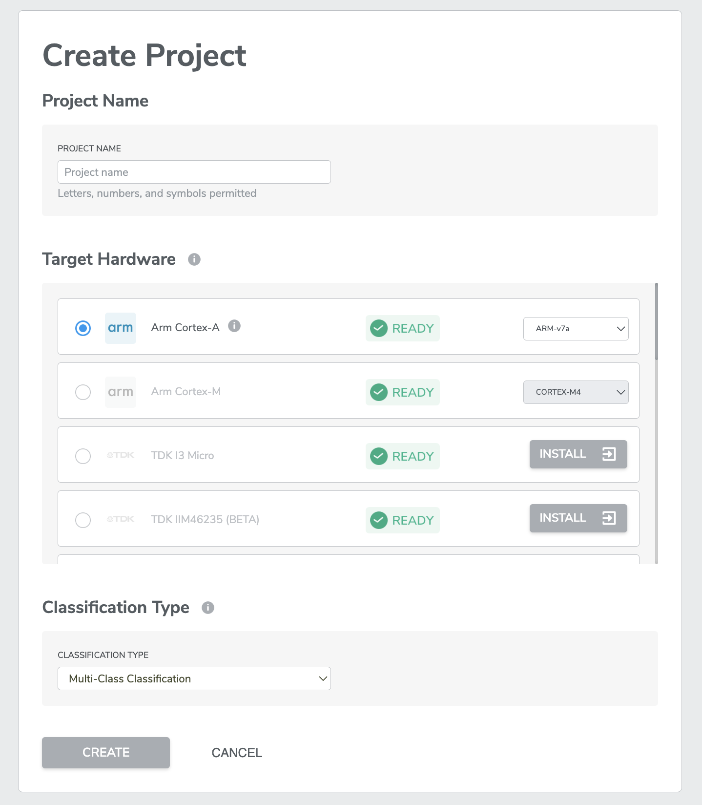
For Cortex-A, users will have to select either ARM_v7a, ARM_v8a_32, ARM_v8a_64 from a dropdown menu on the project creation page, depending on the CPU. The A5, A7, A8, A9, A12, A15, and A17 implement the v7a architecture. The A32, A34, A35, A53, A57, A72, and A73 implement the v8a architecture. Either v8a-32 or v8a-64 should be selected depending on whether the application's execution state is 32-bit or 64-bit.
For Cortex-M, users will have to select either Cortex-M4, Cortex-M7, Cortex-33, Cortex-55 from a dropdown menu on the project creation page, depending on the CPU.
There are few restrictions regarding the type of data that would feed into the model.
Currently the data format is .csv format to upload.
Upload up to 10 files at a time with a maximum size of 70 MB each.
To Start with the Process-
Current supported Cortex-A & Cortex-M:
AVH Corestone Support |
|---|
Cortex-M4 |
Cortex-M7 |
Cortex-M33 |
Cortex-M55 |
Ethos U55 (optional) – enabled in advanced settings during training |
Current supported custom sensor data for Cortex-A & Cortex-M:
Sensor | ODR | FSR |
|---|---|---|
Accelerometer | 12.5Hz - 26kHz | 2g-16g |
Gyroscope | 12.5Hz - 26kHz | 125dps-2,000dps |
Magnetometer | 100Hz | N/A |
Microphone | 16kHz | N/A |
Temperature | 12.5 Hz | N/A |
Pressure | 100 Hz | N/A |
Microphone | 16KHz | N/A |
Current | 1850 Hz | N/A |
Custom sensor 1 | 16KHz | N/A |
Custom sensor 2 | 16KHz | N/A |
Custom sensor 3 | 16KHz | N/A |
Custom sensor 4 | 16KHz | N/A |
Custom sensor 5 | 16KHz | N/A |