
Building Machine Learning Models
In this article:
Step 2a: Sensor Selection (applicable to non-MLC projects)
Option 1 - Automatic Sensor and Feature Group Selection
Option 2 - Manual Sensor Selection
Step 2b: Filter Configuration (applicable to MLC projects)
Option 1 - Automatic Filter and Feature Group Selection
Option 2 - Manual Filter and Feature Selection
Step 3a: Feature Selection (applicable to non-MLC projects)
Option 1 - Automatic Feature Selection
Option 2 - Manual Feature Selection
Step 3b: Feature Selection (applicable to MLC projects)
Step 4a: Inference Settings (applicable to non-MLC projects)
Option 1 - Determine automatically
Step 4b: Inference Settings (applicable to MLC projects)
Step 5: Model Selection & Settings
Multi-class Anomaly classification
Advanced setting for ML Static Library Memory Constraint
Model Performance - ML Model / Cross Validation / Latency / Size / Performance Summary…
Testing Model Performance on Test Data
Event Classification (Start/Stop)
Reading Inference from Hardware
Multi-class Classification Project
Single-class Classification Project
Multi-Class Anomaly Classification
Prerequisites
Sensor is already connected with your laptop through USB or bluetooth
Getting Started
Navigate to the Data page to build machine learning models with collected and/or uploaded training data.
Select training datasets that you want to use for building machine learning models by clicking the checkbox at the left of each Datasets.
*Note that the selected Datasets should ideally be from the same Environment, but Qeexo AutoML will allow you to train Datasets from different Environments as long as the selected sensors and Sensor Configuration are identical.
IN DEMO CASE we select all three dataset that we collected (see Collecting data steps at Data Management ).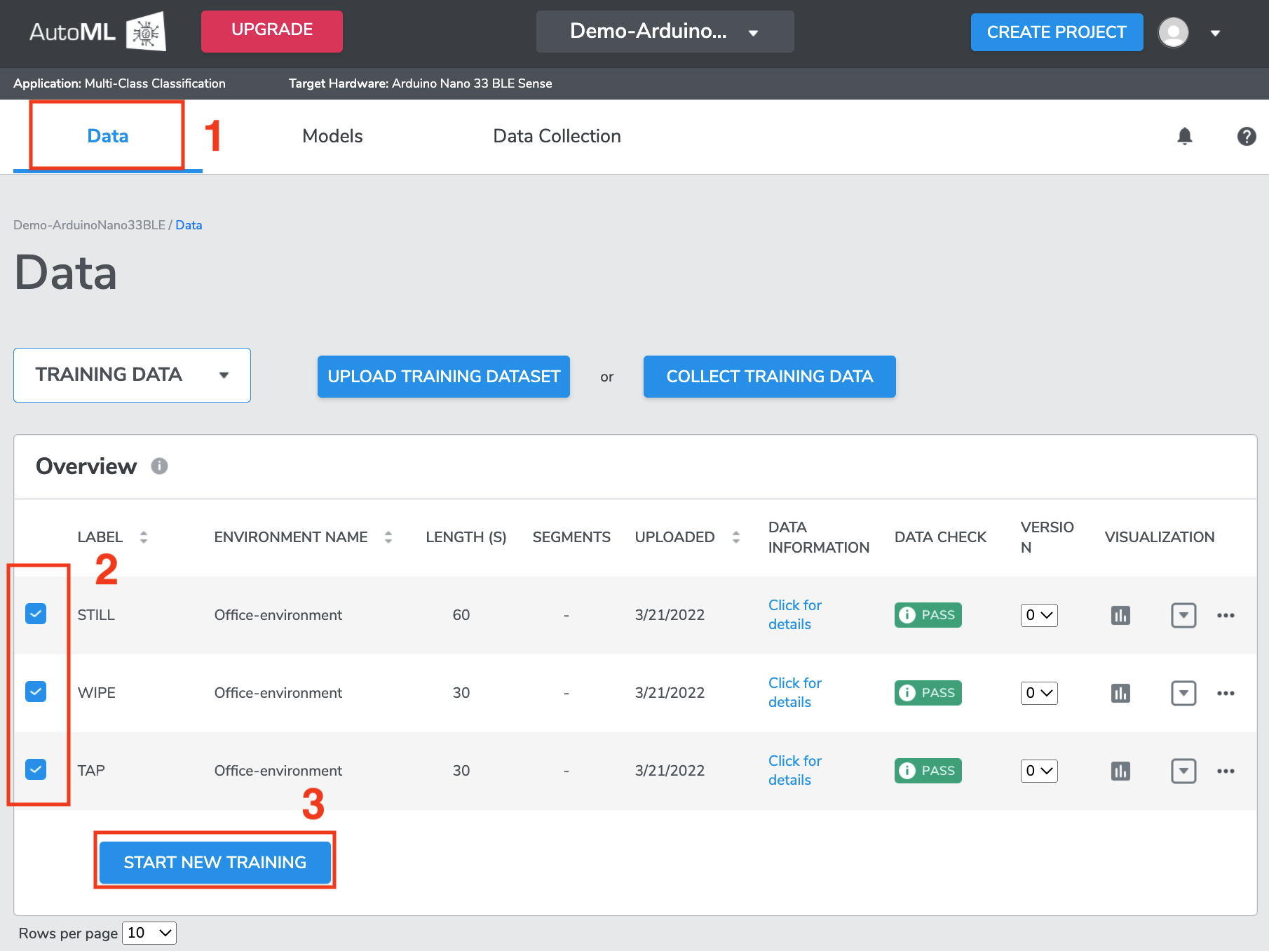
Once the desired Datasets are selected, click
START NEW TRAININGbutton to configure Training Settings.
*Note that theSTART NEW TRAININGbutton is only clickable when Datasets containing 2 or more Class Labels are selected in Multi-class classification project. However, for Single-class classification project, the button becomes clickable as soon as one Class Label has been selected.
*There is a minimum amount of data Qeexo AutoML needs for each Class Label in order to train machine learning models, this minimum is 640 samples from the highest ODR sensor. For example, if your sensor configuration is 104 Hz accelerometer & 25 Hz humidity, you need to collect data for at least 7 seconds (because 104 Hz * 6 seconds < 640 samples). Note that satisfying this minimum requirement does not guarantee performance/accuracy; it is just the minimum amount of data our platform will work with. For good performance, you should likely collect much more than this minimum amount of data.
Training Settings
Step 1: Group labels
This step is an optional step in case you want to group together multiple Class Labels into one Class Label before training the model.
This is an optional step that can be bypassed by pressing the SKIP button.
For example, for a single-class classification project applied to anomaly detection, you may have machinery data that is labelled based on two different types of motion: vertical rotation (UPDOWN) and horizontal rotation (LEFTRIGHT). Since both of these classes are expected behavior, it is convenient to group these labels as a "Normal" group to feed into single-class classification.
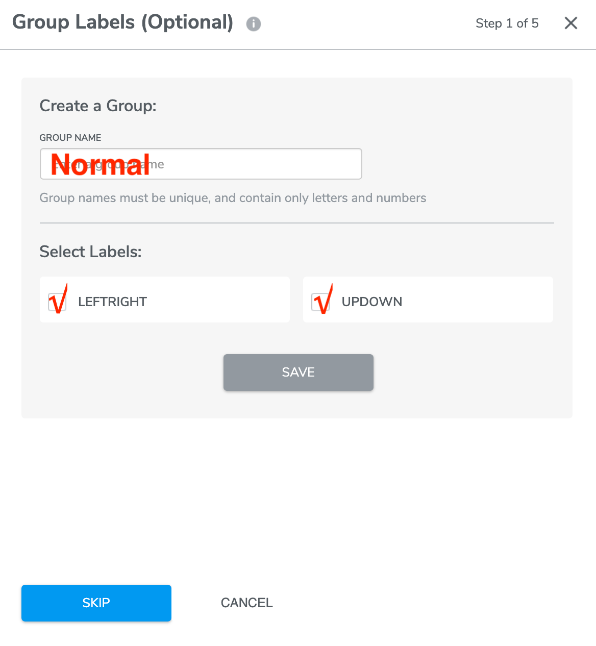
IN DEMO CASE we will skip Group Labels step as we don’t need to.
Step 2a: Sensor Selection (applicable to non-MLC projects)
Step 2a is for projects that is non-MLC project. If you have previously selected MLC for you project, follow Step 2b: Filter Configuration (applicable to MLC projects).
(click Working with Projects for more info regarding creating MLC projects)
There are two options for sensor selection - ‘Automatic Sensor and Feature Group Selection’ and ‘Manual Sensor Selection’.
Option 1 - Automatic Sensor and Feature Group Selection
This is an option to have Qeexo AutoML automatically select sensors and feature groups for optimal model performance. If you have collected data from multiple sensors, but you are not sure which may be helpful for the given problem, it is recommended to enable this feature.
*Note that this automatic selection applies to both sensor and feature groups. If you know what sensors should be used for the problem, but you still want to enable feature selection, that is possible on Step 3a: Feature Selection (applicable to non-MLC projects).
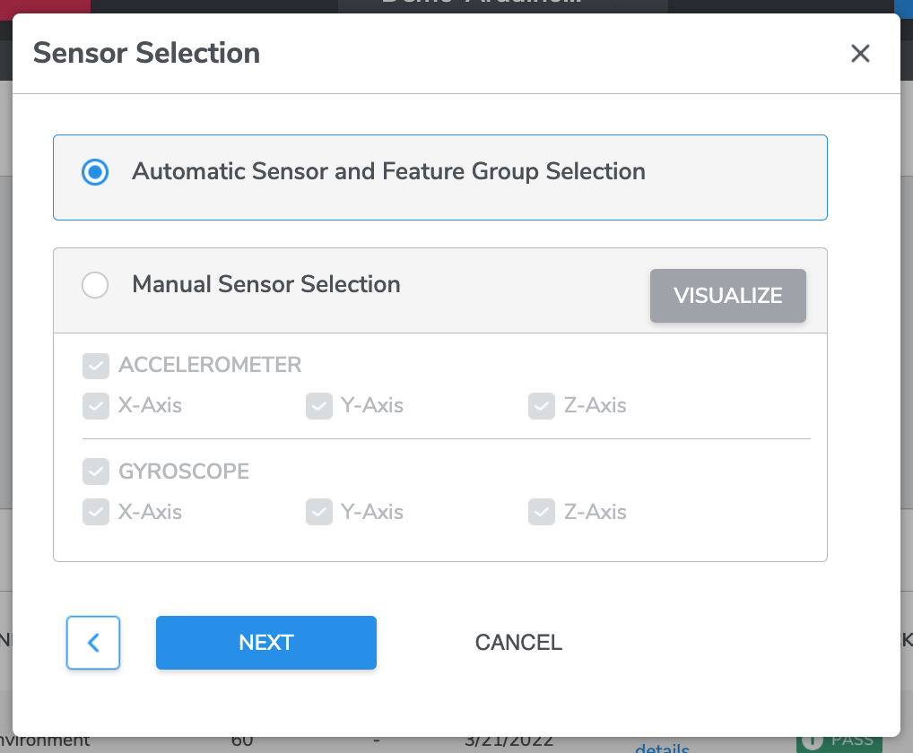
IN DEMO CASE we are going to select “Automatic Sensor and Feature Group Selection”.
Press NEXT when you are ready to proceed to the next step (Please advance to Step 4a: Inference setting (applicable to non-MLC projects)).
Option 2 - Manual Sensor Selection
With manual sensor selection option, you will be able to select a subset of sensor to feed into the Machine Learning pipeline.
*Note that:
All sensors included in Project Creation are available for selection in this stage
Individual axes from multi-channel sensors can be selected independently. These include:
X-, Y-, and Z-axis selection for Accelerometer, Gyroscope, and Magnetometer sensors
Red, Green, Blue and Clear Light channel selection for Ambient Light sensor
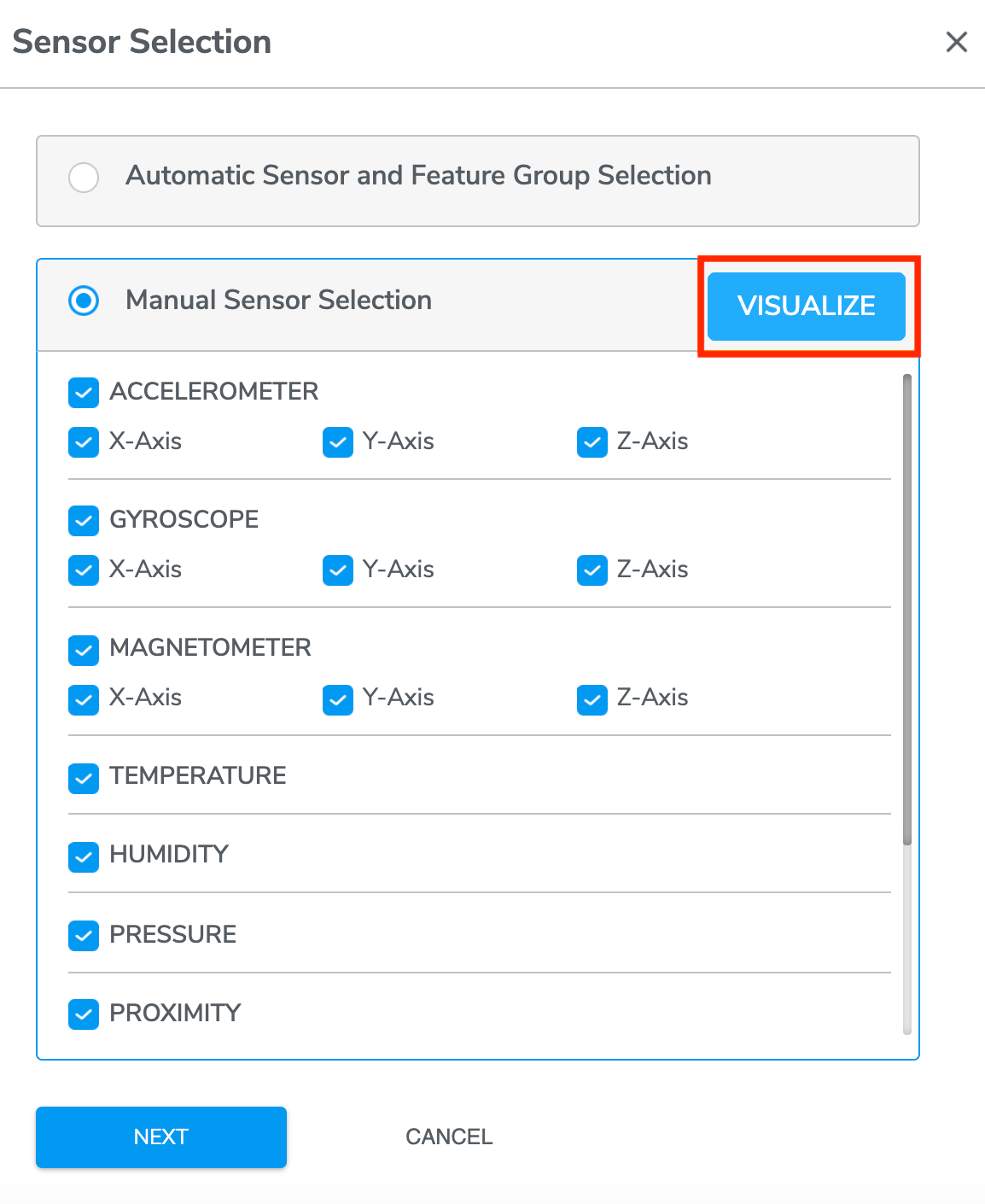
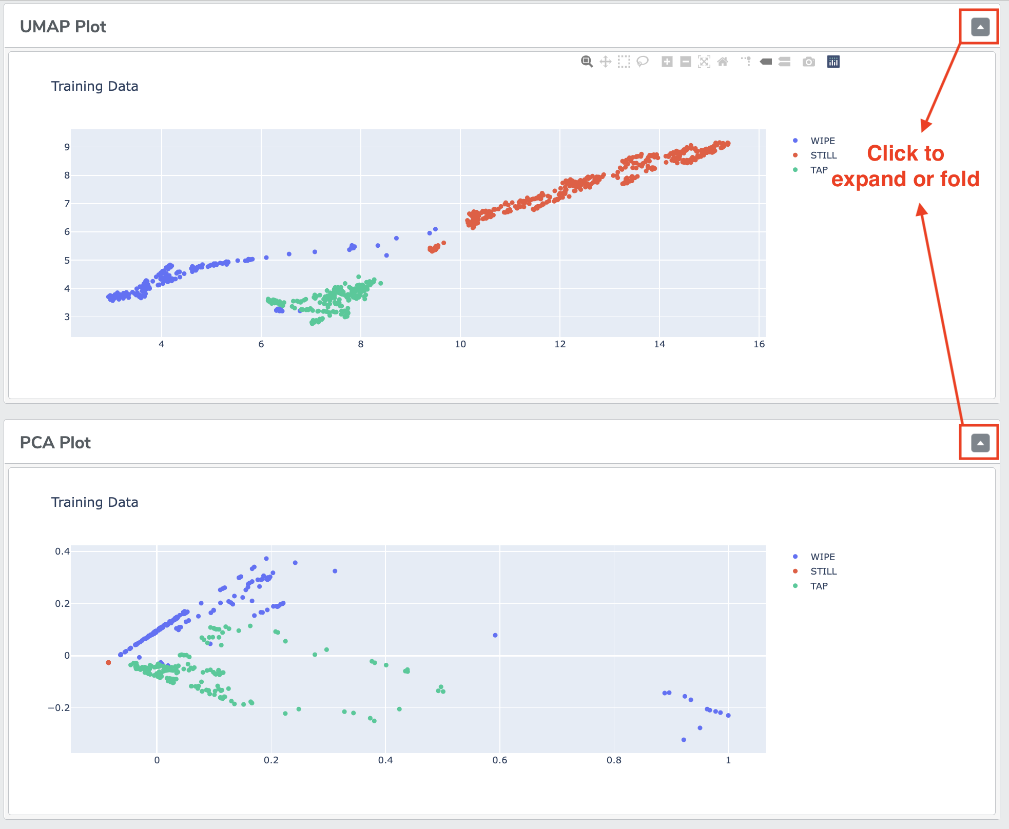
Under manual selection, you can VISUALIZE data collected from sensors using a general-purpose dimensionality reduction algorithms called UMAP (Uniform Manifold Approximation and Projection) and PCA (Principal Component Analysis).
- UMAP is a novel manifold learning technique for dimension reduction. For further details about UMAP algorithm, please refer to "UMAP: Uniform Manifold Approximation and Projection for Dimension Reduction" available at https://arxiv.org/abs/1802.03426 .
- PCA linearly transforms input features into a lower-dimensional space where the variance of the features is maximally preserved. PCA is very well established statistical technique for dimensionality reduction while preserving the variance. Similar to UMAP plot, we project features into two-dimensional space for the PCA visualization as well. These visualizations can often determine which sensors might be useful for classification.
Examining these UMAP and PCA plots before making a final manual sensor selection is encouraged.
Press NEXT when you are ready to proceed to the next step (Please advance to Step 3a: Feature Selection (applicable to non-MLC projects)).
Step 2b: Filter Configuration (applicable to MLC projects)
Step 2b is for projects that is MLC project. If you have previously selected non-MLC for you project, follow Step 2a: Sensor Selection (applicable to non-MLC projects).
(click Working with Projects for more info regarding creating non-MLC projects)
There are two options for Filter Configuration - ‘Automatic Filter and Feature Group Selection’ and ‘Manual Filter and Feature Selection’.
Option 1 - Automatic Filter and Feature Group Selection
If MLC users would like Qeexo AutoML to automatically choose filters and features for their models, select “Automatic Filter and Feature Group Selection” and click NEXT (please advance to Step 4b: Inference Settings (applicable to MLC projects)).
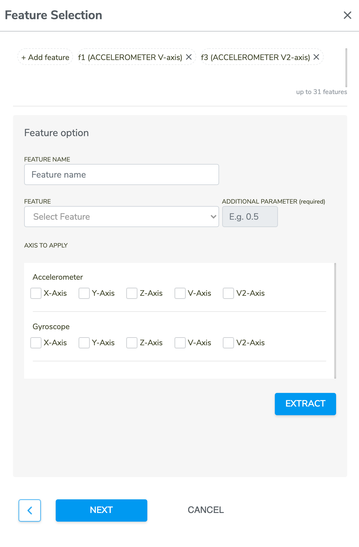
Option 2 - Manual Filter and Feature Selection
For the users who want to manually select filters, they can choose "Manual Filter and Feature Selection" and click NEXT.
Users will be able to configure up to 7 filters that are available in Machine Learning Core logic. Currently the following filters are available:
High-pass filter
Band-pass filter
IIR1 filter
IIR2 filter
Note that filter configuration is entirely optional.
According to ST's documentation, the transfer function of the filter is defined as:
where by the relationship between input, transfer function, gain, and output is illustrated like this:
With this understanding, some of the coefficients are configurable depending on the filter type:
Filter type / Coefficients | b1 | b2 | b3 | a2 | a3 | Gain |
|---|---|---|---|---|---|---|
High-pass filter | 0.5 | -0.5 | 0 | 0 | 0 | 1 |
Band-pass filter | 1 | 0 | -1 | Configurable | Configurable | Configurable |
IIR1 filter | Configurable | Configurable | 0 | Configurable | 0 | 1 |
IIR2 filter | Configurable | Configurable | Configurable | Configurable | Configurable | 1 |
For a detailed explanation and example of filter coefficients, please refer to the ST documentation.
Qeexo AutoML allows for filter to be added and removed:
*Note that V2-Axis means sum of squares of x, y, and z-axis (i.e. x^2+y^2+z^2) while V-Axis is the square root of V2-Axis (i.e. sqrt(x^2+y^2+z^2)).
Press NEXT when you are ready to proceed to the next step (Please advance to Step 3b: Feature Selection (applicable to MLC projects)).
Step 3a: Feature Selection (applicable to non-MLC projects)
Note that this step is automatically SKIPPED when "Automatic Sensor and Feature Group Selection" is chosen previously from Step 2a.
When you chose Manual Sensor Selection previously from step 2a, you will be presented options to select between ‘Automatic Feature Selection’ and ‘Manual Feature Selection’.
Option 1 - Automatic Feature Selection
If the “Automatic Feature Selection” option is chosen, Qeexo AutoML will select the optimal set of features based on final model accuracy as input into model training.
Press NEXT when you are ready to proceed to the next step (Please advance to Step 4a: Inference Settings (applicable to non-MLC projects)).
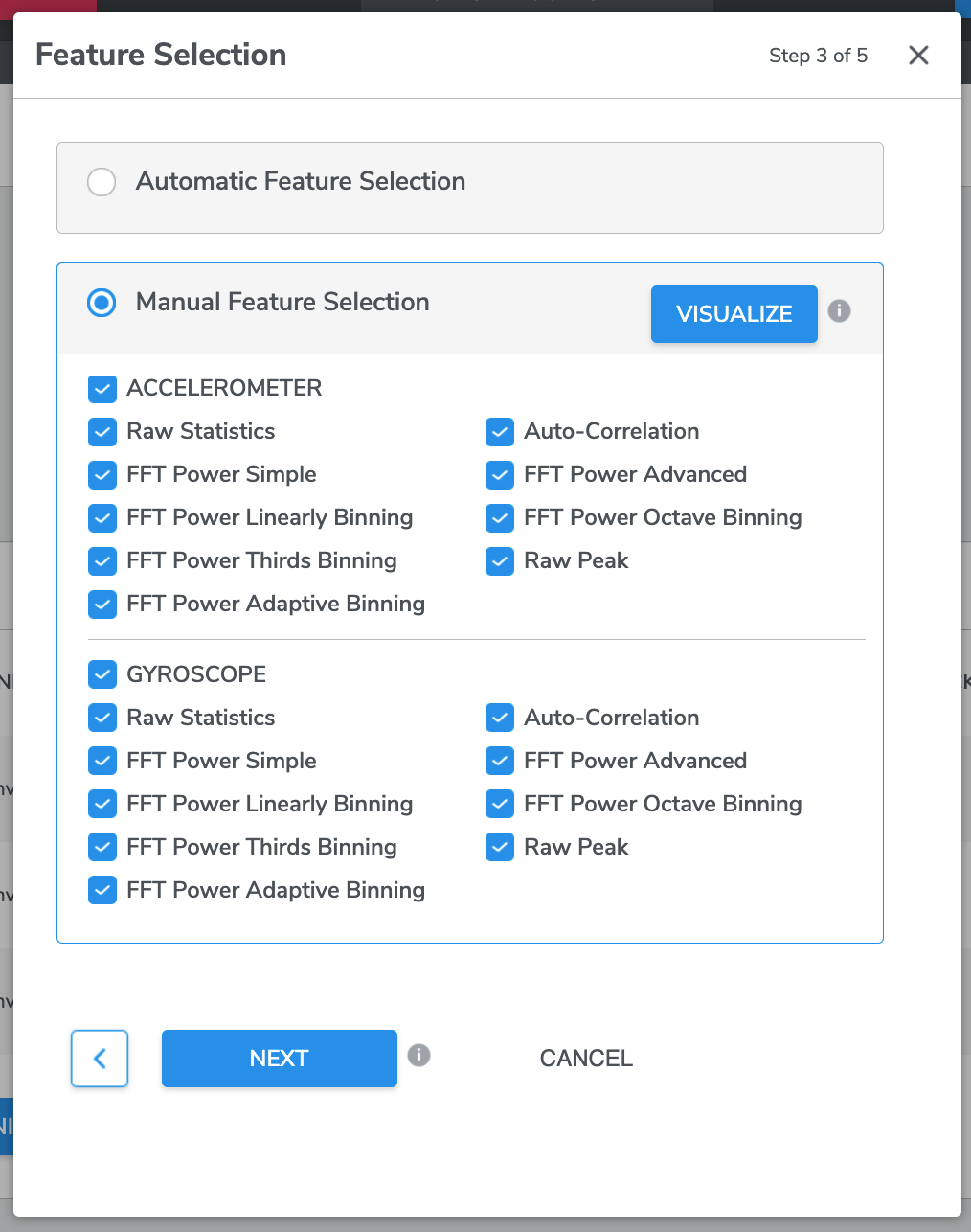
Option 2 - Manual Feature Selection
You may want to refer to the following description of features during Manual Feature Selection:
*Note that features are grouped under each sensor. For each of the selected sensors, at least one feature group is required under the manual mode.
Similar to sensor selection screen, users can visualize data collected from sensors as well as feature groups using the UMAP visualization tool described in the previous section.
Press NEXT when you are ready to proceed to the next step (Please advance to Step 4a: Inference Settings (applicable to non-MLC projects)).
Step 3b: Feature Selection (applicable to MLC projects)
Similar to Step 2b: Filter Configuration (applicable to MLC projects), users can add and remove feature manually.
Refer to ST documentation for more details about the features available in MLC logic.
Press NEXT when you are ready to proceed to the next step (Please advance to Step 4b: Inference Settings (applicable to MLC projects)).
Step 4a: Inference Settings (applicable to non-MLC projects)
There are two options for Inference Settings which are ‘Determine automatically’ and ‘Enter manually’.
Option 1 - Determine automatically
If you select the Determine automatically option, press NEXT to proceed to Step 5: Model Selection & Settings.
IN DEMO CASE After we selected “Automatic Sensor and Feature Group Selection” in Step 2a, here we continue select “Determine automatically” option.
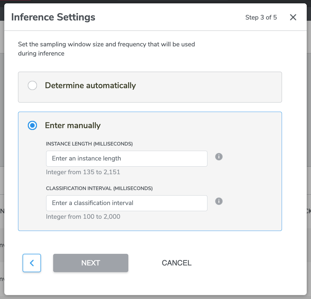
Option 2 - Enter manually
There are two information for you to insert which are “INSTANCE LENGTH (MILLISECONDS)” and “CLASSIFICATION INTERVAL (MILLISECONDS)”.
- INSTANCE LENGTH (MILLISECONDS)
This is sets the length of the sensor data which the model will use to make a prediction, aka what time length of data you would like the model to use to make a prediction. The maximum allowable value for this property is set based on the highest sensor ODR in the given sensor configuration.
The optimal value depends on the real-world time duration of the events corresponding to the Class Labels that you want to capture/detect with the sensors, as well as the selected ODRs used during data collection.
For example, in machine vibration problems, the most important requirement for the signal data is high ODR, because higher ODRs will increase the amount of high frequency information available to the model. For these type of problems, we should often use the highest available sampling rate, and then use the maximum allowable instance length for that ODR (~300 ms @ 6.6kHz).
However, in human activity detection and monitoring, 300 ms would likely not be a sufficient instance length for good performance. We need to make sure the window is long enough to capture some human motion and interaction with the environment, which may require several seconds of data in total. For this case, we should pick an instance length which we want to achieve (e.g. 5000 ms), and then we should use the highest possible ODR which still allows us to achieve this instance length.
- CLASSIFICATION INTERVAL (MILLISECONDS)
This sets the number of milliseconds between requests for classification, aka how often the model makes a prediction once.
For example, if Classification Interval is set to 200 ms, Qeexo AutoML will produce a classifier that classifies incoming data at a rate of 5 Hz.
This value should be set relative to the average time between class changes in the real world -- if the classes may change quickly or last for a very short period of time, Classification Interval needs to be set low so that classifications are run near-constantly in order to capture the events of interest.
For problems like human presence detection, where based on the nature of the problem the classes cannot change often, we may select a higher value (e.g. 2000 ms) in order to save on power consumption and network bandwidth.
Once you are ready, press NEXT to proceed to Step 5: Model Selection & Settings.
Step 4b: Inference Settings (applicable to MLC projects)
MLC has two attributes affecting model inference: ‘Window length’ and ‘MLC output data rate’.
(1) Window Length
All the features are computed within a defined time window, which is called Window length. It represents number of samples, ranging from 1 to 255. Depending on the pipeline configuration, the allowed range for the Window Length may be subject to further restrictions to ensure a minimum number of training instances are created per class label.
(2) MLC Output Data Rate
This parameter governs how fast MLC outputs classification result. Four rates are available: 12.5 Hz, 26 Hz, 52 Hz, and 104 Hz. This parameter must be less than or equal to the Inertial Measurement Unit (IMU) output data rate (ODR). When the MLC ODR is less than the IMU ODR, the sensor data will be downsampled inside the MLC to the MLC ODR before being used in the machine learning model.
Once you are ready, press NEXT to proceed to Step 5: Model Selection & Settings.
Step 5: Model Selection & Settings
This page is for you to select which model type(s) are trained. We are going to discuss steps with respect of different Classification Type - including ‘Single-Class Classification’, ‘Multi-Class Classification’ and ‘Multi-Class Anomaly Classification’. Please refer to your previous selected “Classification Type” for your project.
For multi-class classification, it also contains switches for enabling a few different features related to model building.
Note that only one model (Decision Tree) is available for MLC projects.
A. Single-Class Classification
1. Algorithm Selection
For Single-Class Classification, Qeexo AutoML supports the following machine learning algorithms
*Selecting more than one type of algorithm is recommended, so that results could be compared.
Select the algorithm(s) you want to train the model by clicking the Switch button. You can chose one or more algorithms.
Then click START TRAINING to proceed to Training Process.
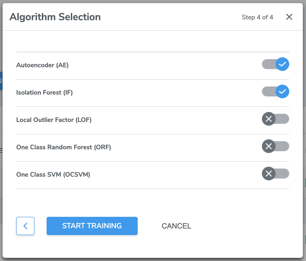
B. Multi-Class Anomaly Classification
1. Algorithm Selection
For Multi-Class Anomaly Classification, Qeexo AutoML supports the following machine learning algorithms
*Selecting more than one type of algorithm is recommended, so that results could be compared.
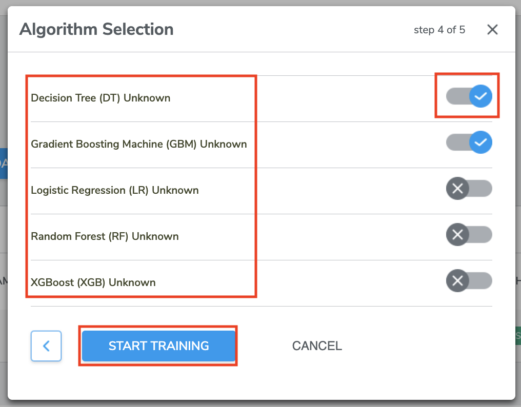
Select the algorithm(s) you want to train the model by clicking the Switch button. You can chose one or more algorithms.
Then click START TRAINING to proceed to Training Process.
C. Multi-Class Classification
1. Algorithm Selection
For Multi-Class Classification, Qeexo AutoML supports the following machine learning algorithms
*Selecting more than one type of algorithm is recommended, so that results could be compared.
Support for additional algorithms will be added in the future
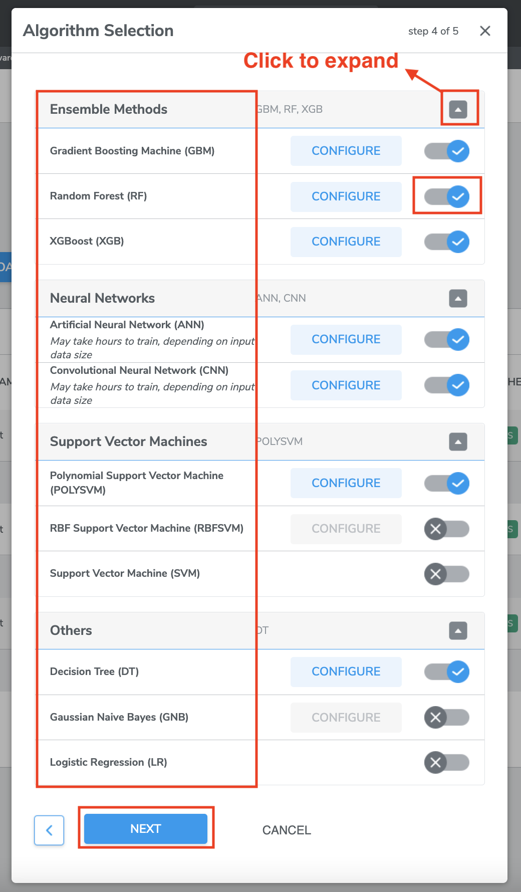
*Note that Neural Networks models may take longer to train, due to the significant computation required for the training process.
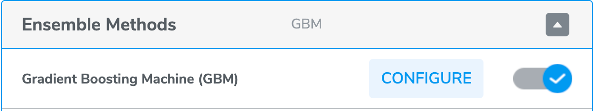
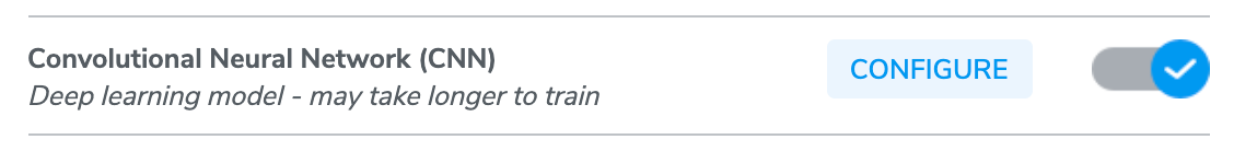
*Additional - the CONFIGURE button
Note: many of these parameters interact with each other in unique and non-intuitive ways. Unless you have significant experience tuning deep learning models, you may want to consider using the automatic hyperparameter optimization tool.
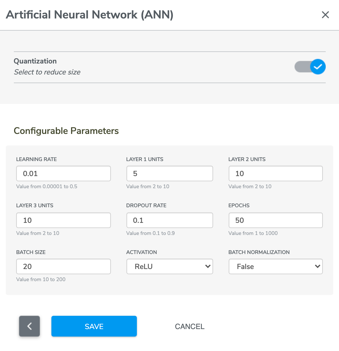
Pressing CONFIGURE (available for some models) will yield the following configuration screen:
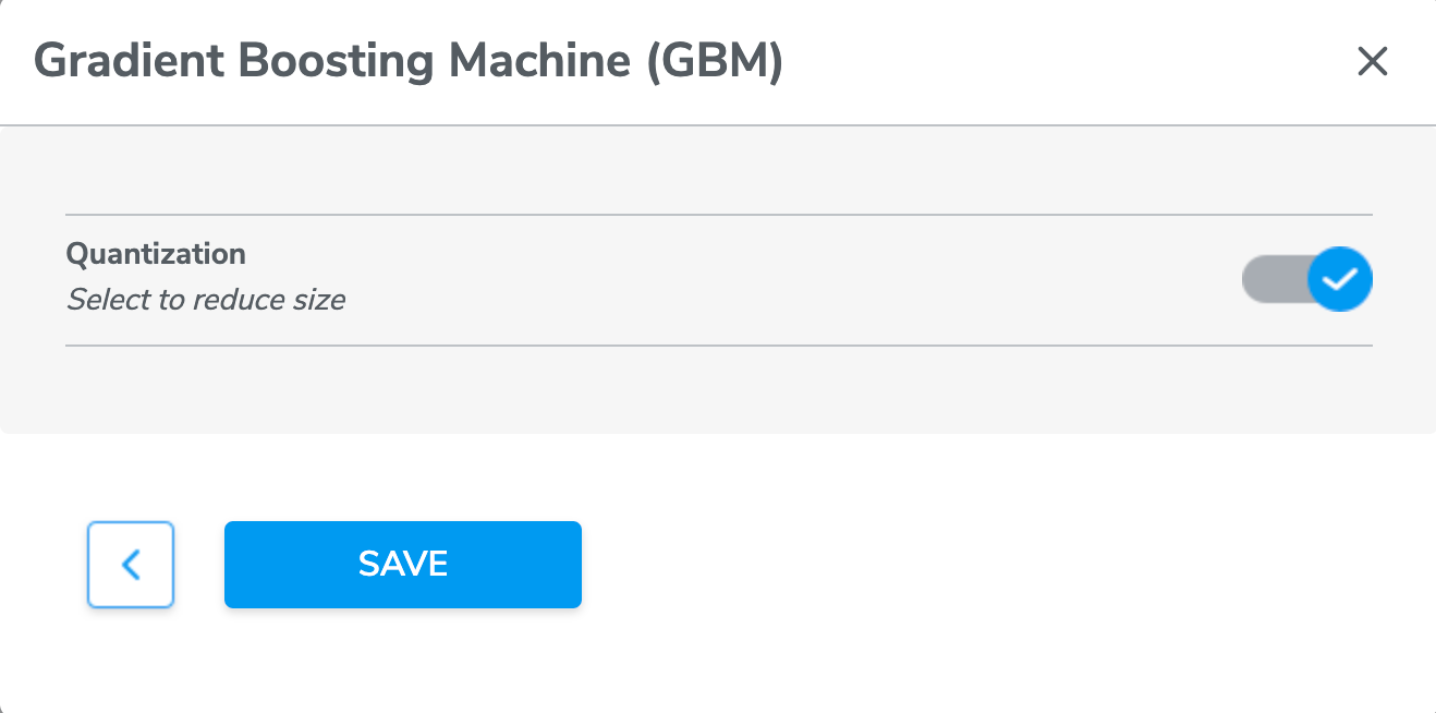
Quantization denotes an option to conduct quantization - aware training so as to achieve model size reduction.
There are additional configurable options to fine tune the ANN model
Configurable Option | Description |
|---|---|
Learning rate | Scaling parameter which sets the step size at each iteration in optimization of the cost function |
Layer 1 units | Number of nodes in layer 1 |
Layer 2 units | Number of nodes in layer 2 |
Layer 3 units | Number of nodes in layer 3 |
Epochs | Number of passes through the complete training dataset; one epoch means the network will use each training instance exactly once |
Dropout rate | Fraction of units to drop during each training round, applied to all network layers |
Batch size | Number of training examples in one training round; higher batch sizes may have faster runtimes, but are more likely to get stuck in local optima |
Batch normalization | If true, apply normalization process to the output of each layer, typically helpful for improving the convergence and stability of the training process |
Activation | Function applied to the outputs of the neurons |
Similarly there are configurable options to fine tune the CNN and RNN model
Configurable Option | Description |
|---|---|
Tensor Length limit | Threshold length that determines whether to stop adding convolution layers (reducing the length limit will lead to more convolution layers) |
Learning rate | Scaling parameter which sets the step size at each iteration in optimization of the cost function |
Batch size | Number of training examples in one training round; higher batch sizes may have faster runtimes, but are more likely to get stuck in local optima |
Dense layer units | Number of nodes in the final network layer |
Dropout rates | Fraction of units to drop during each training round, applied to all network layers |
Epochs | Number of passes through the complete training dataset; one epoch means the network will use each training instance exactly once |
Input layer filters | Number of filters in the first convolution layer |
Intermediate layers filters | Number of filters in all the intermediate convolution layers |
Input layer strides | Number of samples to move at each step along one direction for the first convolution layer |
Intermediate layers strides | Number of samples to move at each step along one direction for all intermediate convolution layers |
Augment | If true, apply data augmentation technique to prevent overfitting; will lead to higher training time due to larger amount of data |
Batch normalization | If true, apply normalization process to the output of each layer, typically helpful for improving the convergence and stability of the training process |
Activation | Function applied to the outputs of the neurons |
Input layer kernel size | Filter kernel size in the first convolution layer |
Intermediate kernel size | Filter kernel size in the all intermediate convolution layers |
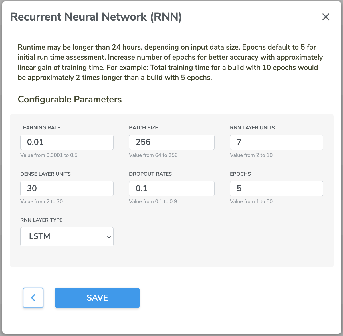
Configurable Option | Description |
|---|---|
Learning rate | Scaling parameter which sets the step size at each iteration in optimization of the cost function |
Batch size | Number of training examples in one training round; higher batch sizes may have faster runtimes, but are more likely to get stuck in local optima |
Dense layer units | Number of nodes in the final network layer |
Dropout rates | Fraction of units to drop during each training round, applied to all network layers |
Epochs | Number of passes through the complete training dataset; one epoch means the network will use each training instance exactly once |
Configuration sub-menu for other algorithms will be added in the future
Select the algorithm(s) you want to train the model by clicking the Switch button. You can chose one or more algorithms.
Then click NEXT to proceed to Model Settings.
IN DEMO CASE We are going to select all available algorithms, then click NEXT to proceed to Model Settings page.
2. Model Settings
There are two parts in Model Settings page for you to select and input information which are ‘Generate Learning Curve(s)’ and ‘Hyperparameter Tuning’.
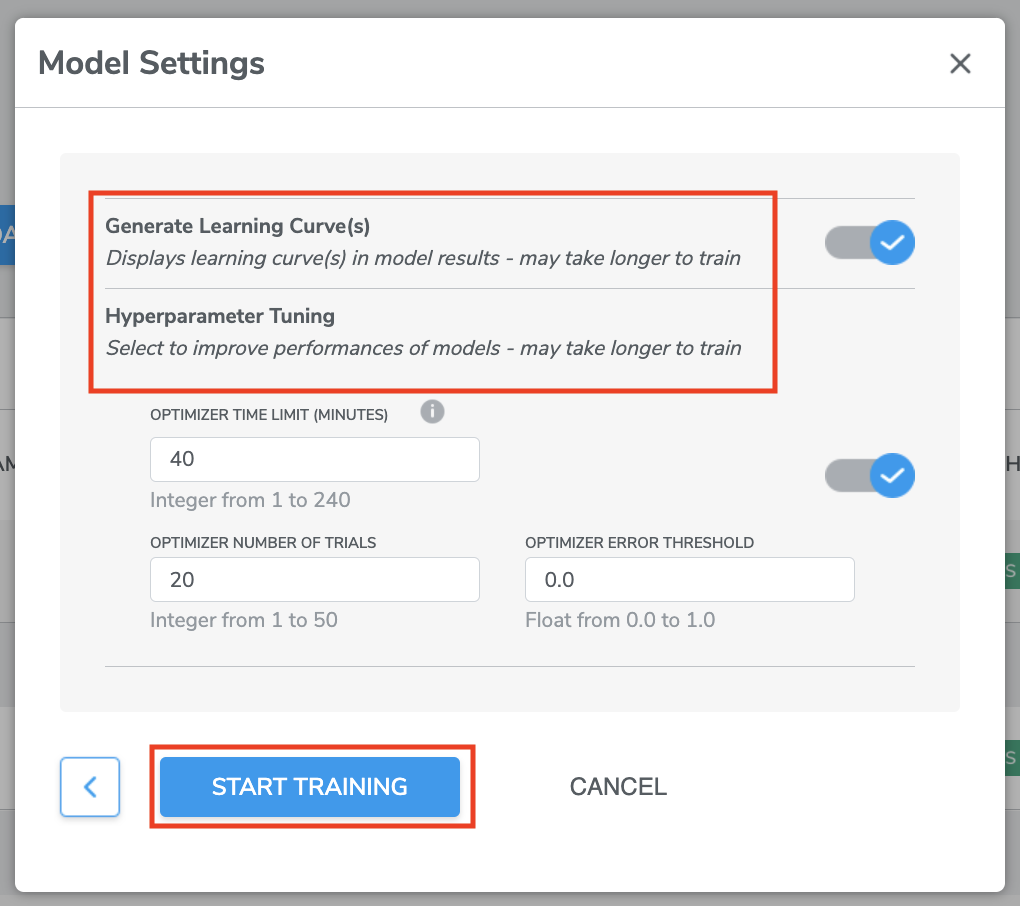
(1) Generate Learning Curve(s)
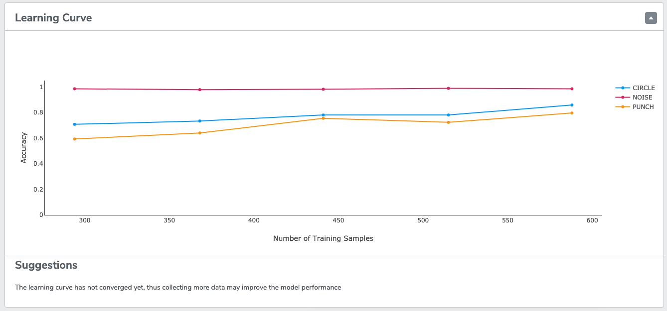
If enabled, this option will produce learning curves for the given data set. Learning curves visualize how your model is improving as more data is added. These curves can be extrapolated, which can be useful for determining if the model may benefit from additional data collection.
As shown in the example below, the "Circle" and "Punch" gestures are still improving with additional data. It is likely that they would continue to improve if more data is collected.
*Note: If the dataset that is used for training is very small, the learning curves may not be accurate. The model may be very good at classifying the limited data it's seen, but might not generalize to new cases. In that case, even if the learning curve does not show it, it is safe to assume that final model performance will improve with additional data collection.
(2) Hyperparameter Tuning
Hyperparameters are a set of adjustable parameters of machine learning models. These parameters affect the accuracy, runtime, and size of machine learning models. Different models have different parameters depending on the model architecture. AutoML provides built-in option for tuning these hyperparameters. There is a simply switch users need to flip if hyperparameter optimization is desired. If this option is enabled, AutoML tunes hyperparameter using a collection of optimization techniques tailored to TinyML applications. It maximizes accuracy while it ensures that all resource usages are under constraints (e.g., firmware binary size and memory usage). This option will often improve final model accuracy at the expense of additional runtime for model-building.
There are three settings that affect the duration of the hyperparameter tuning stage:
- Optimizer Time Limit:
- Optimizer Number of Trials:
- Optimizer Error Threshold:
Once you are ready, click START TRAINING to proceed to Training Process.
IN DEMO CASE For Model Settings, we will leave everything as default, simply click START TRAINING to proceed.
D. Advanced setting for ML Static Library Memory Constraint
When Pro Tier users select data collections and continue to click START NEW TRAINING button to start the model training, we added a new advanced option to allow users to configure ML Static Library Memory Constraint, more specifically, users could set the target ML Static Library maximum flash and RAM memory size usage as desired.
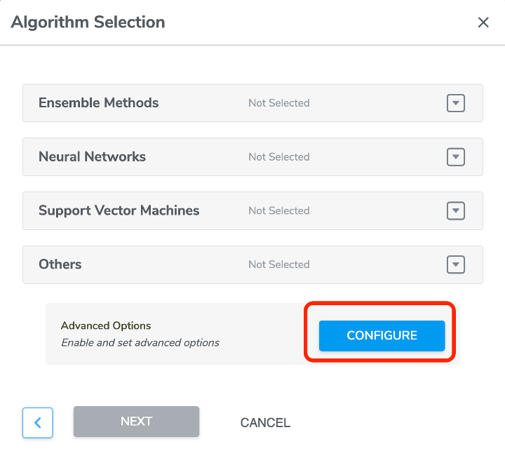
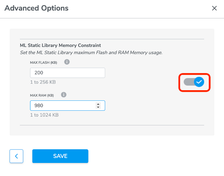
In the Algorithm Selection window, user could click CONFIGURE button to access to the Memory Constraint feature. The toggle on the right side should be enabled before users type in any values in the field on the left side.
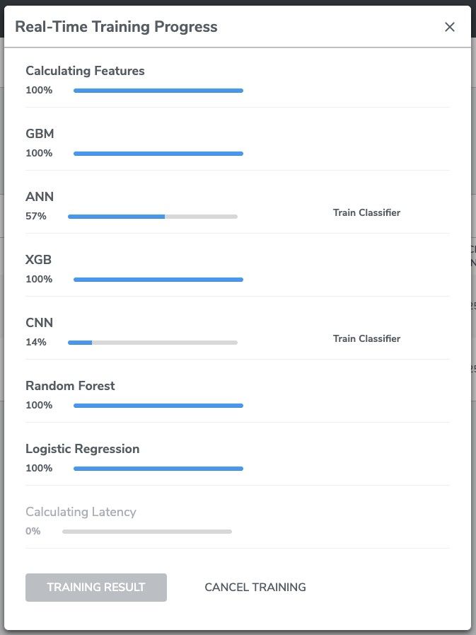
Training Process
Once you clicked "START TRAINING" with one or more selected machine learning algorithms, the training process will begin.
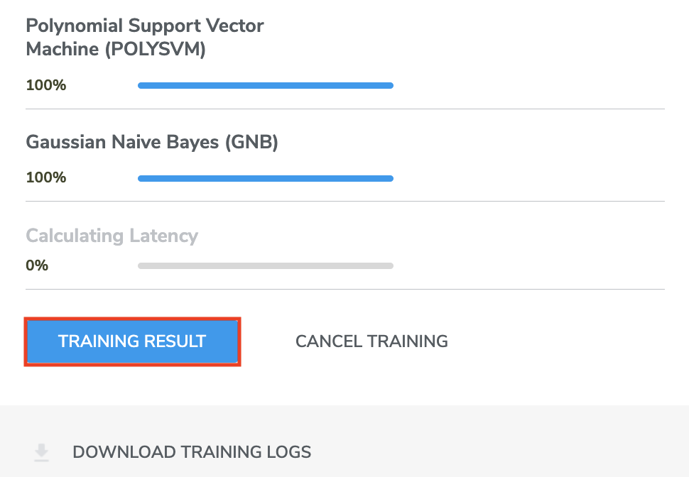
Real-Time Training Progress pops up after training begins. The top row shows the progress of common tasks (e.g. featurization, data cropping, etc.) shared between different algorithms, followed by the build progress of each of the selected models.
At the end of the training process, Qeexo AutoML will flash, in sequence, each of the built models to the hardware device to test and measure the average latency for performing classifications.
Training Result
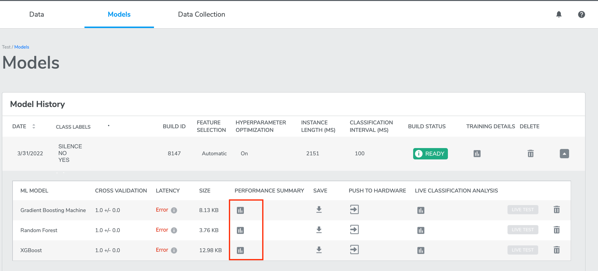
Click "TRAINING RESULT" to navigate to the Models page (also reachable from the top navigation bar), where all of the previous trainings will be listed, with the most recent one on top.
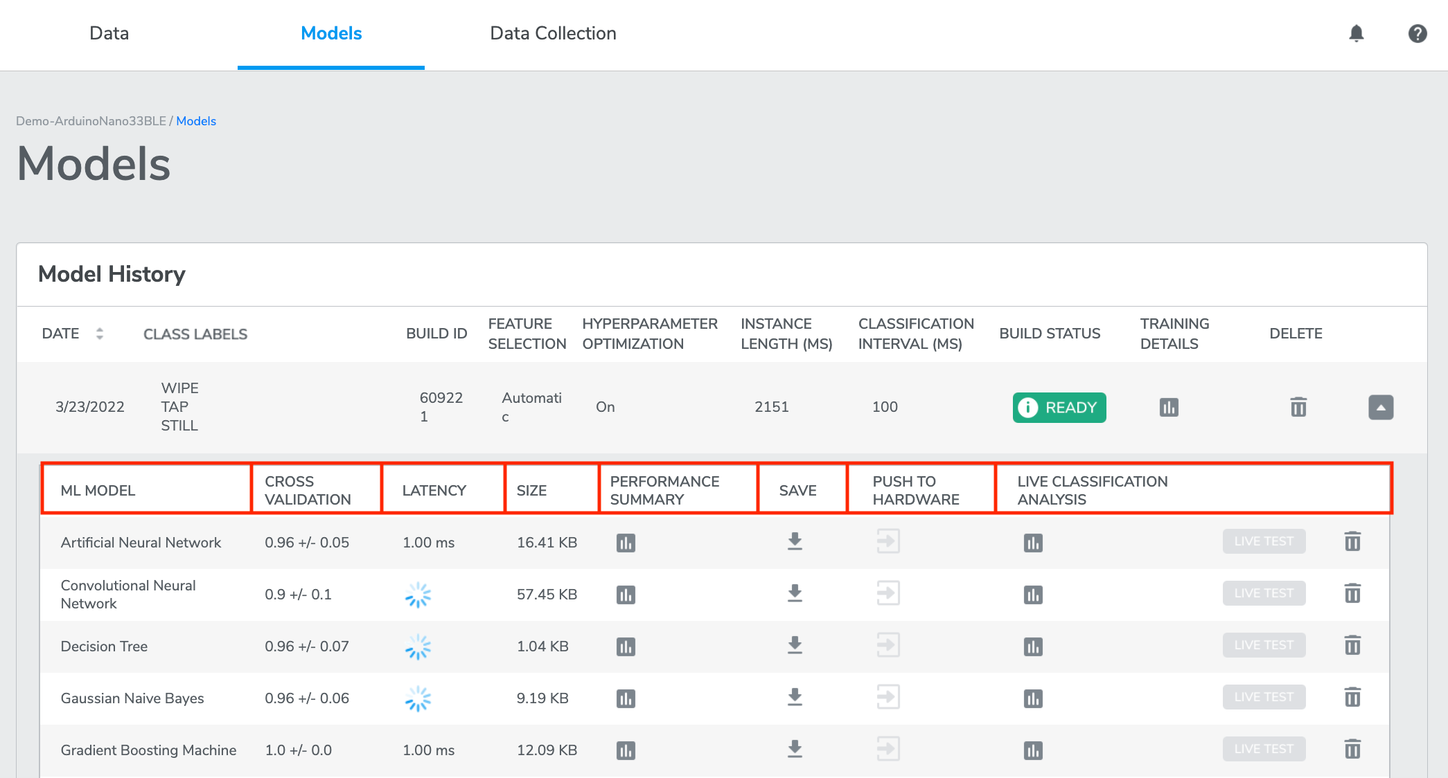
The current training will be expanded to show relevant information about model performance, including ML MODEL (the type of machine learning model), CROSS VALIDATION accuracy, LATENCY, SIZE, and additional PERFORMANCE SUMMARY. It also allows you to SAVE each model to your computer, PUSH TO HARDWARE (push a selected model to Target Hardware for LIVE TEST), LIVE CLASSIFICATION ANALYSIS and DELETE the model.
ML MODEL - Each entry is differentiated by the algorithm with which each model had been built. We also call these machine learning "packages" because they include supporting code such as sensor drivers in addition to the machine learning models built by Qeexo AutoML.
CROSS VALIDATION - This is the average classification accuracy for 8 different models, each trained and tested on different, mutually-exclusive subsets of the given data.
*This is always a value between [0, 1], with 0 being the worst accuracy and 1 being perfect accuracy.LATENCY - Latency is the average time (in milliseconds) required for the machine learning model to compute the prediction of a single instance. It includes time spent on featurization of sensor data and running inference with the model. We calculate this average empirically by first flashing each model to the Target Hardware, running 10 inferences, then taking the average.
*Note that the concept of latency is not applicable to MLC projects.
*The short the value, the better.SIZE - This is the memory size of the model parameters and the model interpreter. The model interpreter executes the model parameters in combination with the sensor readings to provide the model results. This measure gives an idea of the impact of this model to on-device memory usage in comparison to other models trained on the same data.
Consider the following notes to understand the ML Model Size measurement:
- None of the model size measurements include the sensor data processing and featurization code. That can add 10KB – 20KB to the size of the final library for all models except raw-data-based models (CNN, CRNN, RNN)
- The static library output from AutoML may be larger than the size reported due to the featurization code as well as other necessary interface utilities
- The binary used for flashing to the device for Live Testing from AutoML will be significantly larger as it also must include other system libraries for the target platform - The concept of memory size with MLC projects does not apply as the decision tree is implemented in hardwarePERFORMANCE SUMMARY - Press "PERFORMANCE SUMMARY " to bring up a pop-up window with additional information about each of the machine learning models.
*Note that the amount of model details depends on whether the project is for single-class or multi-class classification.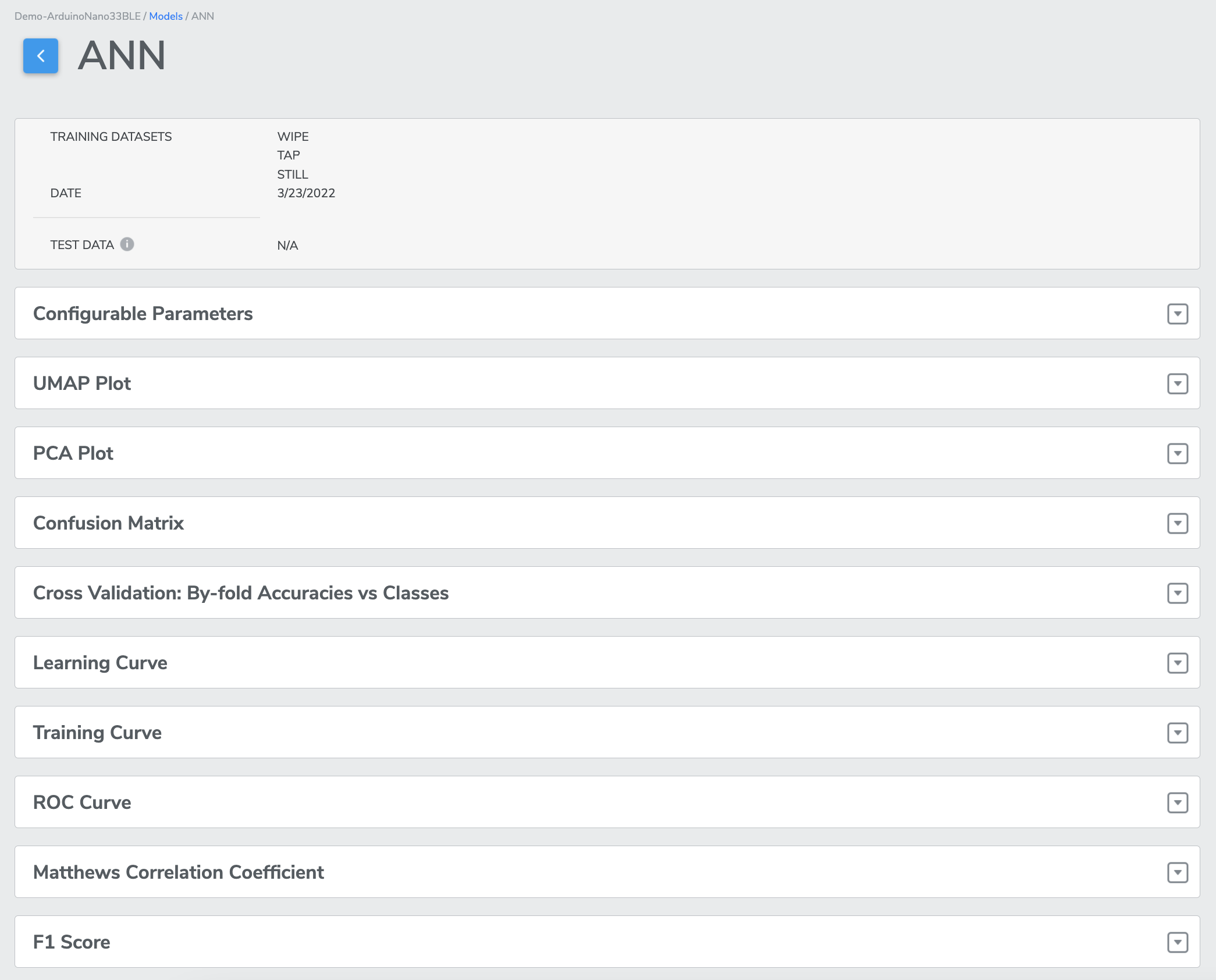
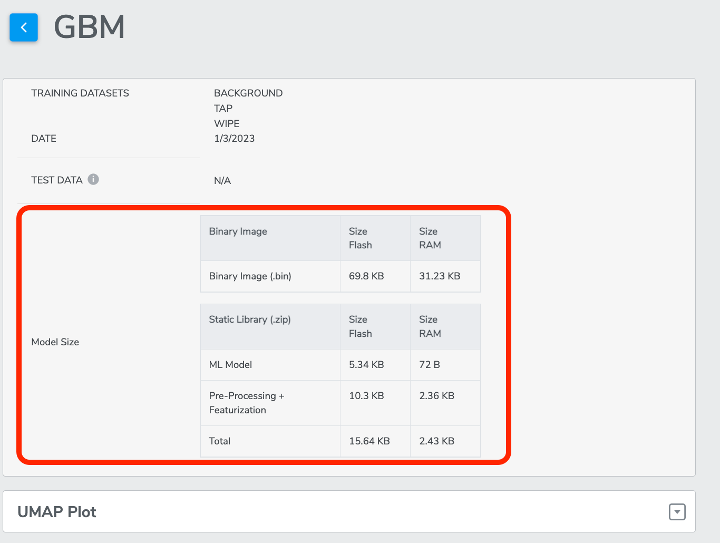
Report on size taken by ML Model and Other code separately per ML library built under Model page
From here, users could check the flash and RAM size of binary image, ML model, pre-processing + featurization and the total size. The very basic benefit is that it brings more model information for users to use as a reference when selecting final model. We are sure it also provides more flexibility and possibilities per user case.
Multi-class classification
UMAP and PCA Plots: we are showing the dimensionality reduction UMAP and PCA plots as visual indications of how the training datasets are "clustered" in the given model.
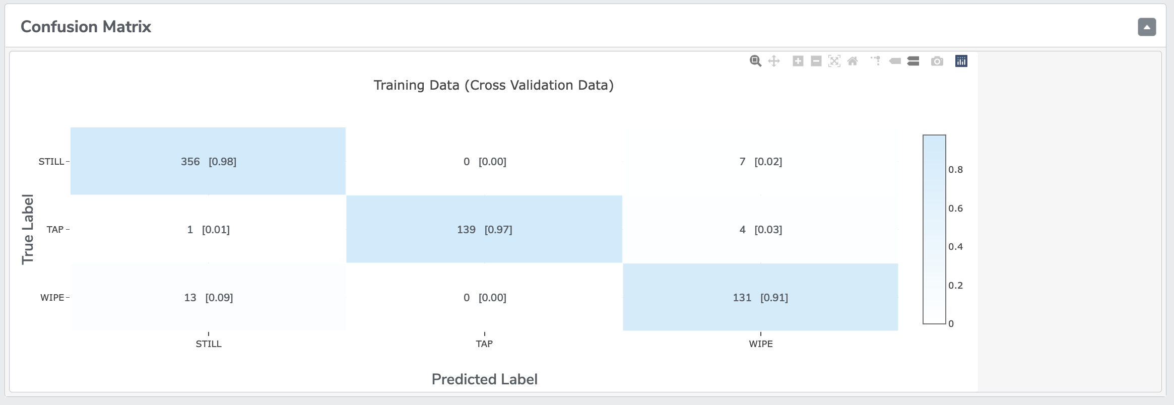
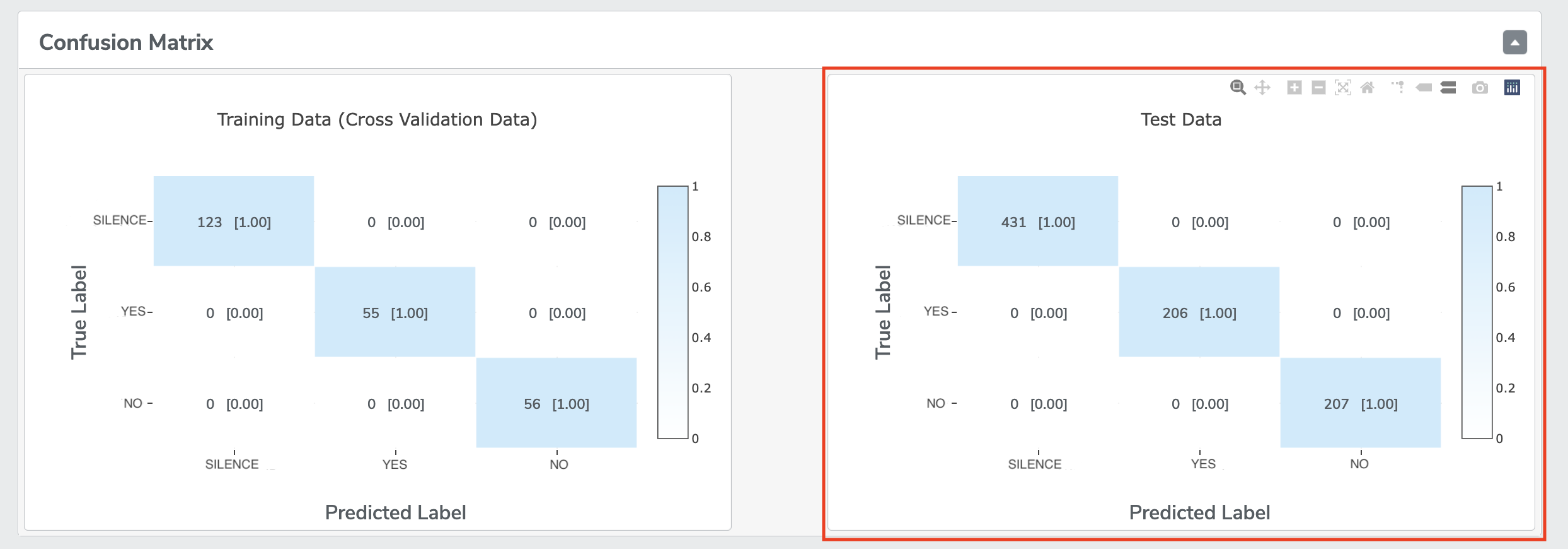
Confusion Matrix: it represents True Labels and Predicted Labels. Diagonal (upper left to lower right) elements indicates instances correctly classified. Off-diagonal elements indicate instances mis-classified. Summing instances over each row should sum to total instances for the respective class. For Multi-Class Anomaly Classification, there will be an extra unknown class label.
Cross Validation: By-fold Accuracies vs Classes: it represents the spread of classification accuracies across the CV folds. This representation is done by-class. If the by-fold points are all shown close to the mean line, this shows that the average by-class accuracy is a precise measurement of how well the model should perform for the given class. More variance in the by-fold points suggests that the model may perform much better or much worse than expected.
Learning Curve: it illustrate the performance for each class at different number of instances of data collected/uploaded. Each point on the Learning Curve is the cross-validation accuracy at the respective data size. This gives an understanding of whether adding more data will help to improve the classification performance for each class and whether similar performance can be achieved with fewer instances of data.
ROC Curve: RoC Curves plot the False Positive Rate (FPR, x-axis) vs. True Positive Rate (TPR, y-axis) for each class in the classification problem. The dotted line indicates flip-of-the coin performance where the model has no discriminative capacity to distinguish between 2 classes. The greater the area under the curve (AUC), the better the model.
Matthew's Correlation Coefficient (MCC): it is a measure of discriminative power for binary classifiers. In the multi-class classification case, it can help show you which combinations of classes are the least well understood by your model.
* The values can range between -1 and 1, although most often in AutoML the values will be between 0 and 1. A value of 0 means that your model is not able to distinguish between the given pair of classes at all, and a value of 1 means that your model can perfectly make this distinction. For Multi-Class Anomaly Classification, there will be an extra unknown class label.
There will be one MCC value for every pair of class labels in the datasets (order does not matter). For example, there will be 3 coefficients for each combination of the 3 class labels, and 6 coefficients for 4 class labels.F1-Score: F1-score factors false positives, false negatives, and true positives. F1-score thus is an important model performance metric. Accuracy only can obscure some important aspects of model performance if a large proportion of a dataset belongs to one class. In contrast, F1 score is more tolerant to this type of class imbalance problems. Operating the model at the peak of the F1-score means the rate of True Positives and False positives are optimized. To the either side of this point, either True positives or False positives dominates.
*F1-score also lies within the unit interval (0-1]; the best score is 1, and it approaches 0 as performance gets worse.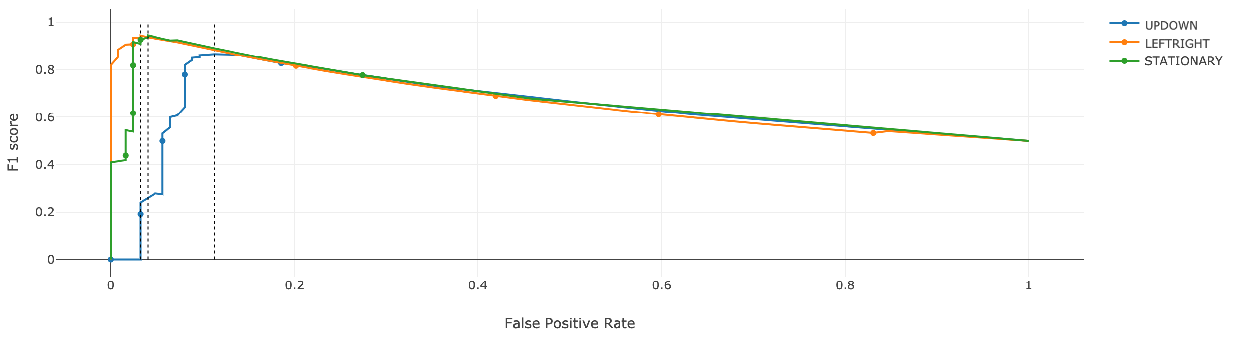
Single-class classification
Confusion Matrix: For the single-class classification case, we only have data from the one given class. A perfect confusion matrix for single-class models has all of the cases concentrated in the top-left corner, meaning that none of the given class data was classified as not coming from that class.
Cross Validation: By-fold Accuracies vs Classes: Similar to the confusion matrix case, the most important information in the single-class classification by-fold results are the left-most case. This will show us how varied our single-class accuracies were for each fold of our cross validation.
Matthew's Correlation Coefficient: For single-class classification, there is only one Matthew's Correlation Coefficient, which measures the quality of the classification between the given class and things that do not belong to the given class.
*The values can range between -1 and 1, although most often in AutoML the values will be between 0 and 1. A value of 0 means that your model is not able to recognize the given class at all, and a value of 1 means that your model can perfectly make this distinction.
SAVE
For non-MLC projects, there are 2 options"Save .bin" - download the model as a binary image to your machine.
"Save .zip" - download a compressed archive of header file and static library whereby users can build custom application on top of the machine learning model.
For MLC projects, users can ONLY save the MLC configuration of the model as
jsonfile.PUSH TO HARDWARE - Flashes the model to the Target Hardware.
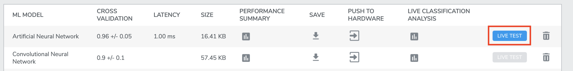
*Target Hardware must be connected.LIVE TEST - Once the model has been PUSH TO HARDWARE, "LIVE TEST" becomes clickable, and will take you to Live Testing Page.
DELETE - When a model is no longer required, you can delete it. A confirmation dialog box will be presented.
LIVE CLASSIFICATION ANALYSIS
Sensitivity Analysis
*Note that there is no sensitivity analysis for single-class projects.
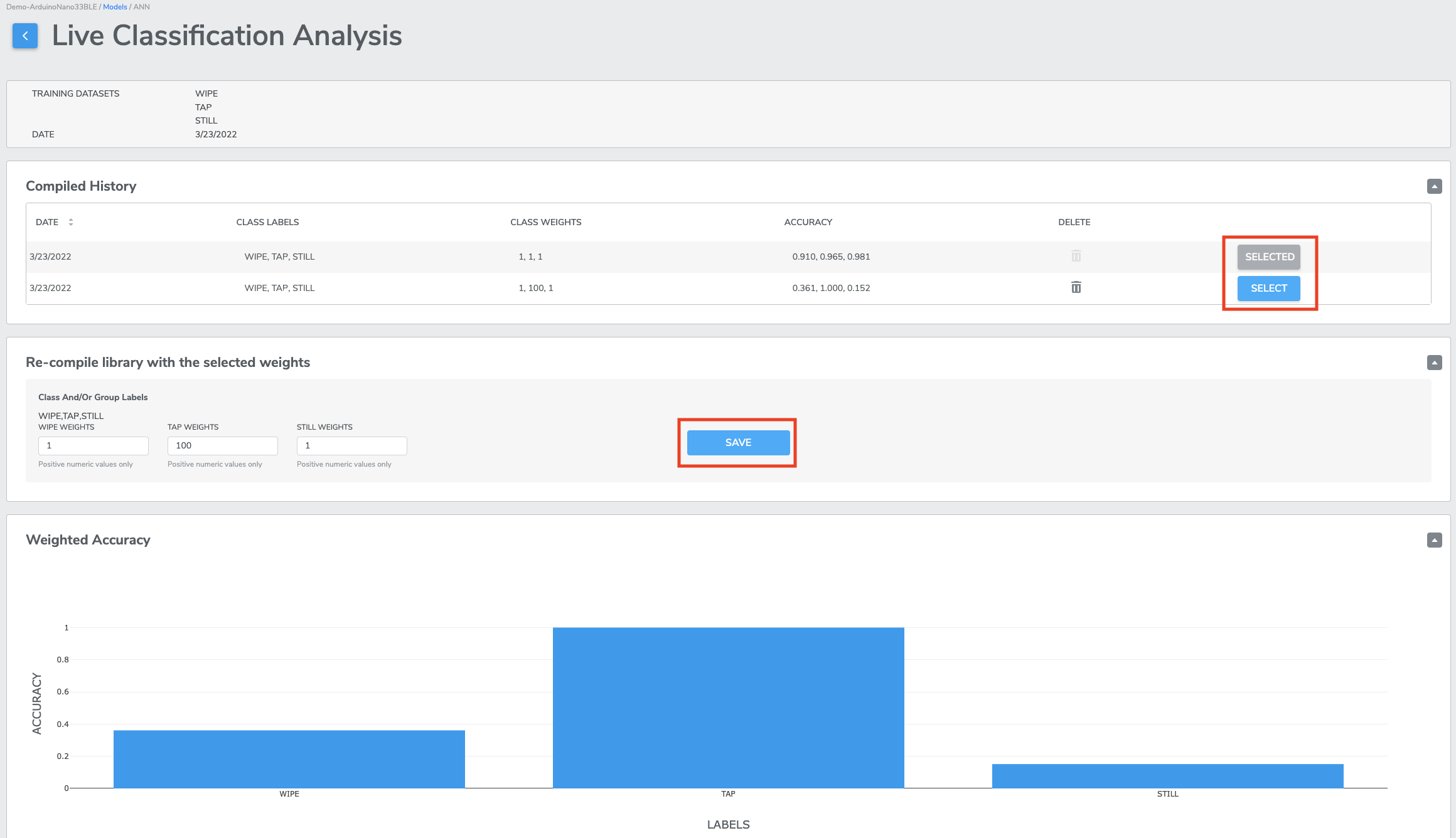
For multi-class classification, the Sensitivity Analysis tool allows you to trade off accuracy between classes, depending on your specific use-case. You can re-weight the classes in your model and see how the cross-validation accuracies and confusion matrix is affected.The selected sensitivities are normalized and are used to scale the model output probabilities. Higher values for a given class will make the model more likely to ultimately make a classification of that type.
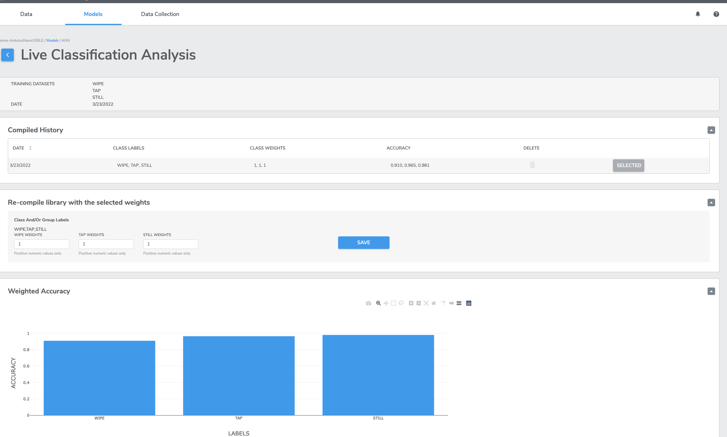
The easiest way to understand how the Sensitivity Analysis page works is to train a multi-class model and then try a few different values. The accuracy plots and confusion matrix will update in real-time along with your changes to the sensitivities. Notice how the plots change when the sensitivity for the "Punch" class is increased from 1 to 100:
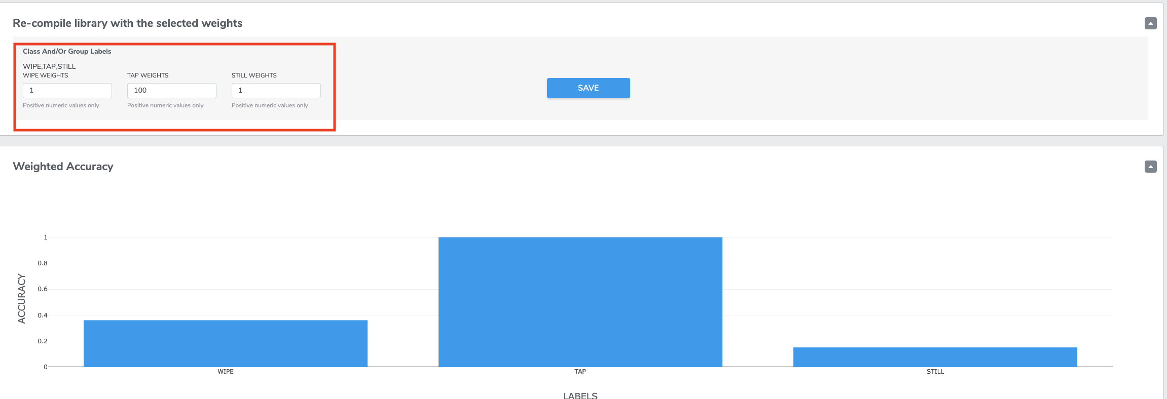
Once you find sensitivity values that seem best for your use-case, press "SAVE" on the new sensitivity values. This will generate a new binary with your selected values. Click "Select" on the newly-compiled binary, and this updated binary will be the one that is flashed to your device when you go to test live classification.
Live-Data Collection and Analysis
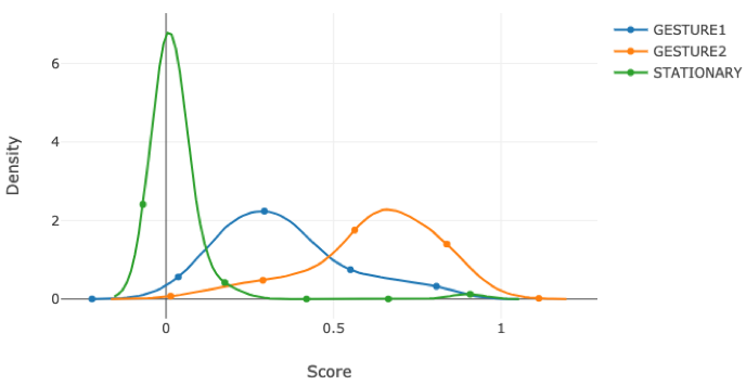
Live-data collection allows users to collect the live data for specific duration, class-by-class and then the subsequent analysis section shows a confusion matrix, ROC curves, Matthews correlation coefficient, and F1 score. Moreover, AutoML estimates the distribution of prediction scores using kernel density estimation (KDE).KDE plots provide detailed insights into error analysis. The example below is a KDE plot for a gesture recognition problem. All instances are collected as "Gesture2". Ideally, the scores for the other classes should be distributed around zero. However, the mode of "Gesture1" distribution (the blue line) is 0.3, and its tail extends beyond 0.5. These signify potential issues with the live-data or the model used for the analysis. We want to see the distribution of "Gesture1" and "Gesture2" as separate as possible with almost no to little overlap for both the classes. While we can observe that the "Stationary" class is quite well separated from "Gesture1" and "Gesture2". "Stationary" class has a peak around zero and also very narrow compared to "Gesture1" and "Gesture2" very well isolates it.
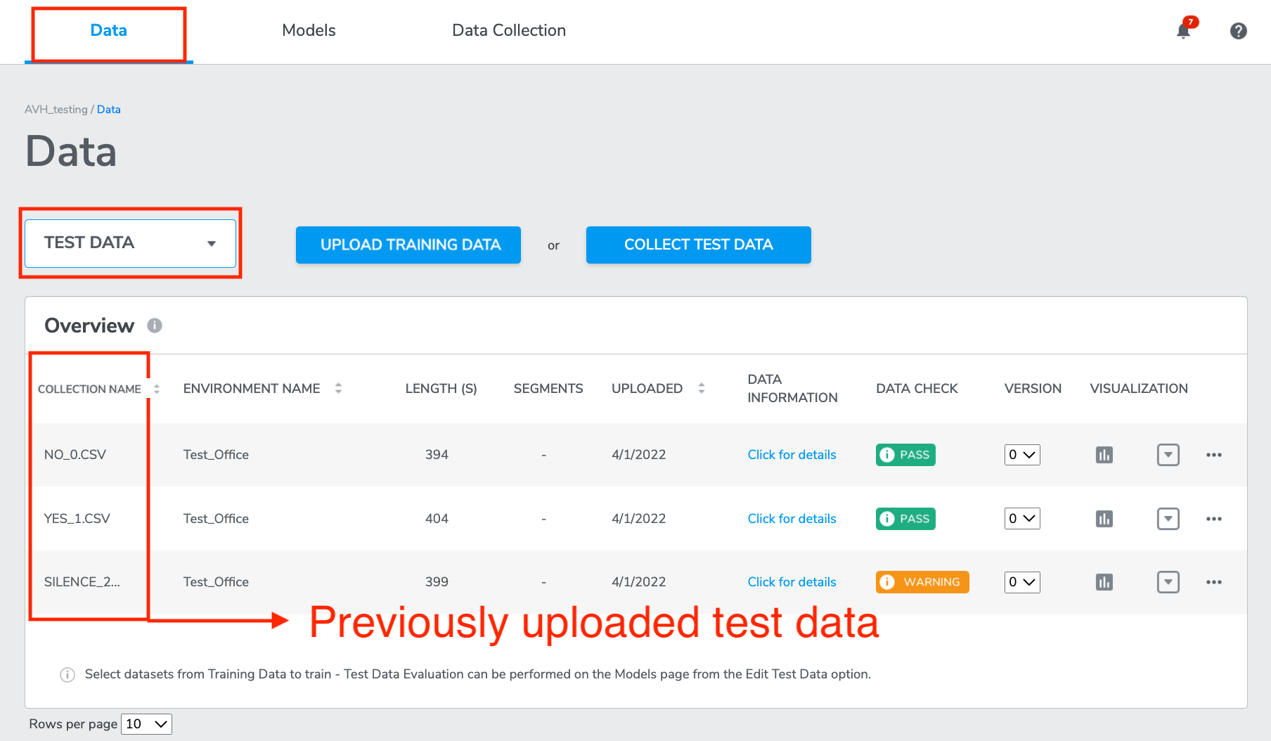
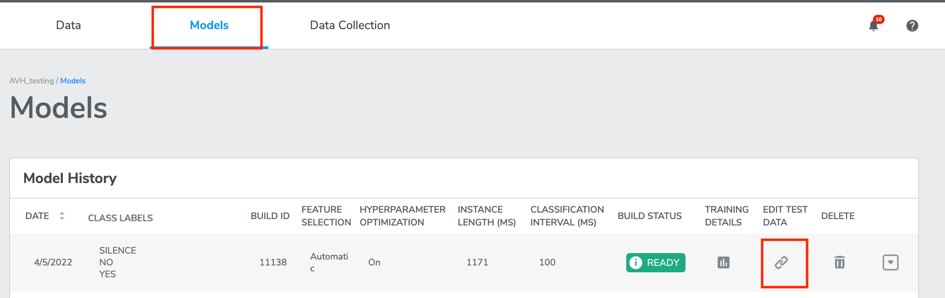
Testing Model Performance on Test Data
You can test all your ML models' performance by using the uploaded test data (if you have previously uploaded test data).
Click the button under EDIT TEST DATA.
A window will pop out. Here Test Data collections on the left may be linked to Training Data collections on the right by clicking the checkbox for the row and selecting the desired training collection form the drop-down.
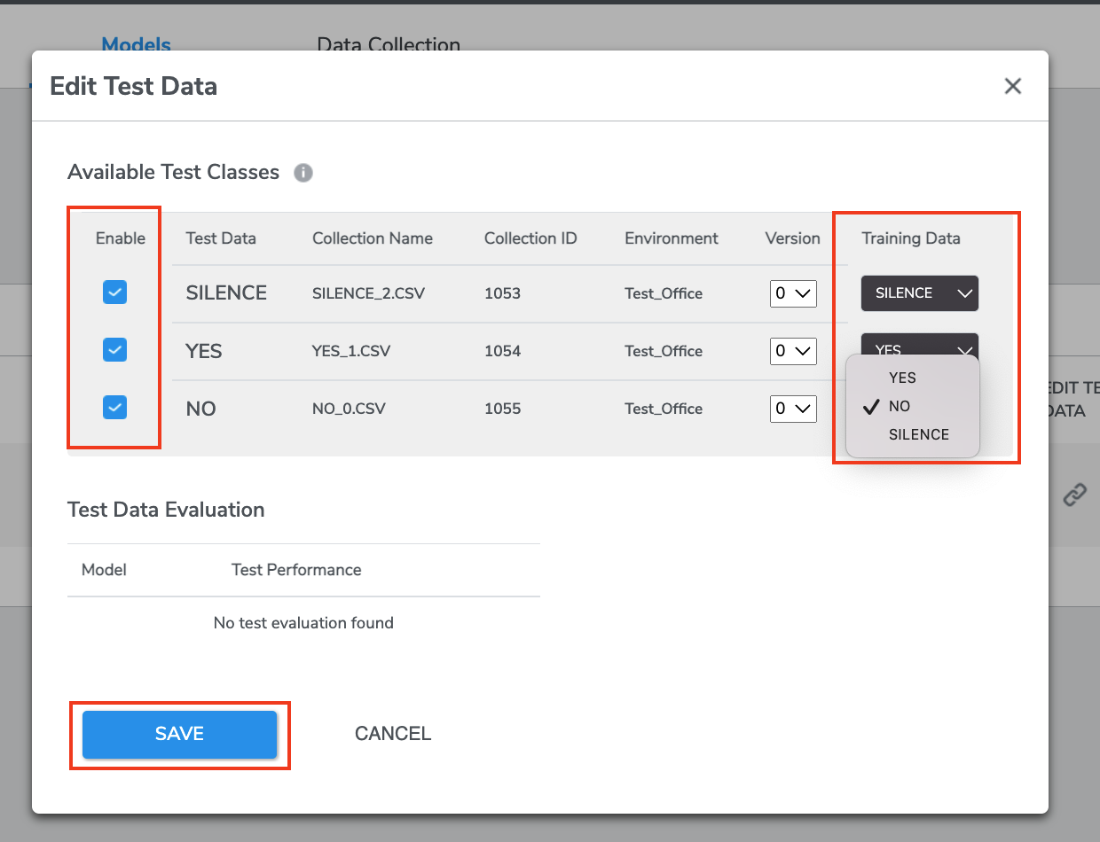
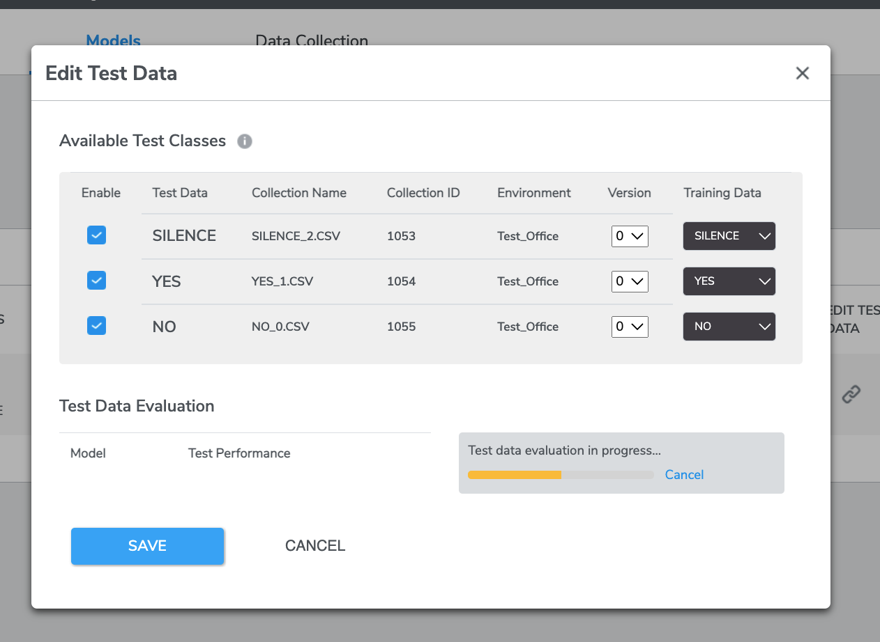
Select at least one data by clicking the check button on the left. Clicking SAVE will dispatch the test run and evaluate the model's performance using the linked test data.
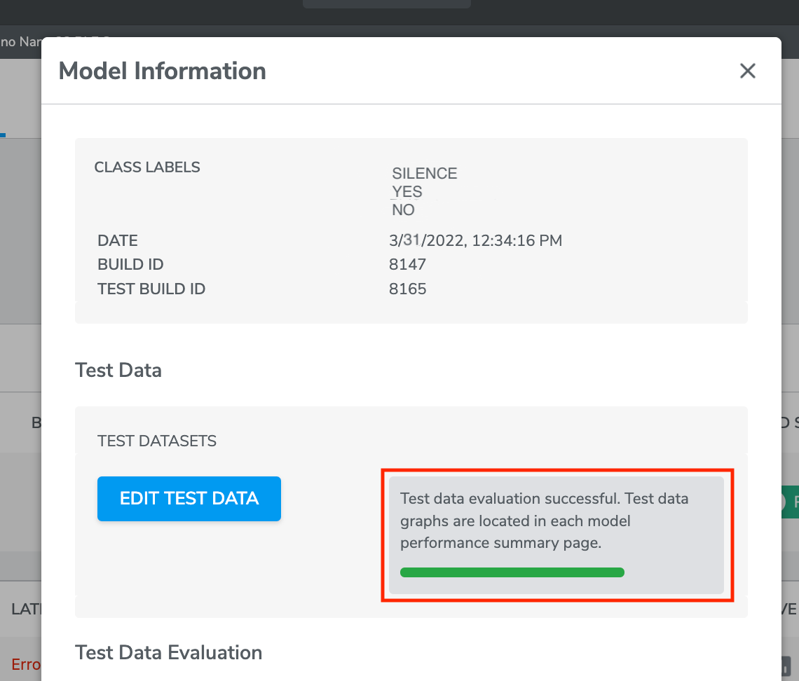
Once the evaluation is completed, you can find the result of Model performance on Test Data by clicking the buttons under “PERFORMANCE SUMMARY” of each model.
Live Testing
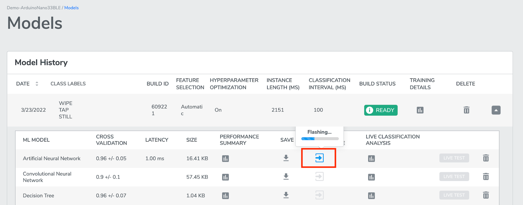
From the Test Result Page, you can select a model out of your interest, click the Arrow button under PUSH TO HARDWARE to flash the model to the Target Hardware. Note that the Target Hardware MUST BE connected to your laptop.
Once the model has been PUSH TO HARDWARE, LIVE TEST becomes clickable, and will take you to Live Testing Page.
Here in the Live Testing page, you can perform live-testing. The screen will display the current class that is predicted by the model that was flashed to the Target Hardware, based on the signals from the enabled sensors for this Project.

Classification Methods
There are two classification methods which are Continuous Classification and Event Classification (Start/Stop).
1. Continuous Classification
Continuous classification is selected on the live test page as default. In continuous classification, the live test screen will display the classification result one after another in a rate you set previously in classification interval. Continuous classification is recommended when the training sets are all continuous data.
A meta-classifier is a filter on the outputs of the decision tree. The meta-classifier uses some internal counters to filter the decision tree outputs. The purpose of the meta-classifier is to reduce false positives, avoid generating an output which is not stable, and reduce the transitions on the decision tree result.
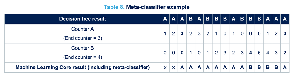
The previous table shows the effect of filtering the decision tree outputs through a meta-classifier. The first line of the table contains the outputs of the decision tree before the meta-classifier. Counter A and Counter B are the internal counters for the two decision tree results (“A” and “B”). In the activity recognition example, the result “A” might be walking and the result “B” jogging. When the internal counter “A” reaches the value 3 (which is the End Counter for counter “A”), there is a transition to result “A”. When the internal counter “B” reaches value 4, there is a transition to result “B”.
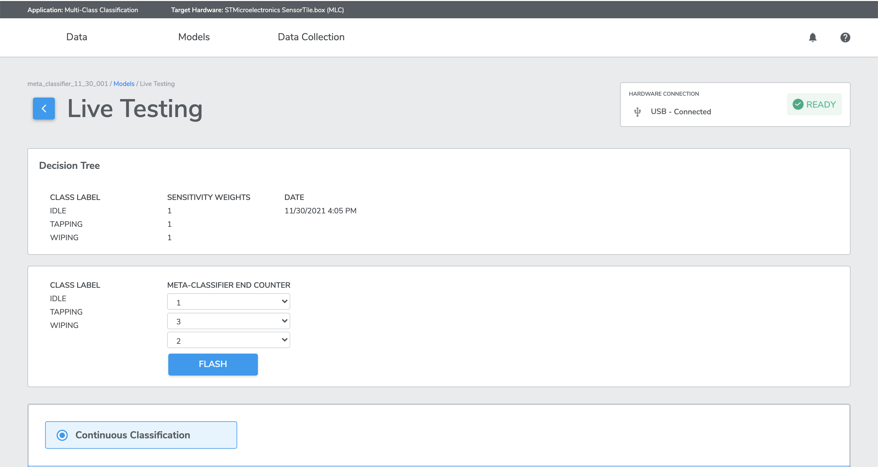
The user can read/edit the meta-classifier end counters in the live testing page of MLC projects. The default values of end counters after flashing MLC model are 0.
The user can update the meta-classifier end counters in the live testing page within acceptable range (0-14). if the users have increased the end counters of a class label, it will take “longer” for MLC to output the classification result for that label, compared to before the change. Say the user increased the end counter for class “drum” from 1 to 5. It will now take more occurrences of “drum” output to reach to 5 than 1, resulting in potentially “longer time” between classification output changes, thus serving the false positive reduction objective. Setting what end counter values are subject to human judgement, depending on ML use cases.
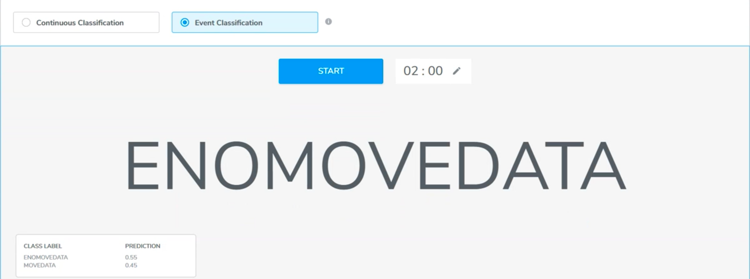
2. Event Classification (Start/Stop)
In event classification, the model will only read the sensor input within the event window, and give one prediction after each event.
Event classification is recommended when the training set contains segments.
Using GUI button: Press START and begin performa the event. The prediction result will display on the screen after the event ends by either pressing STOP or the n second of event length is up.
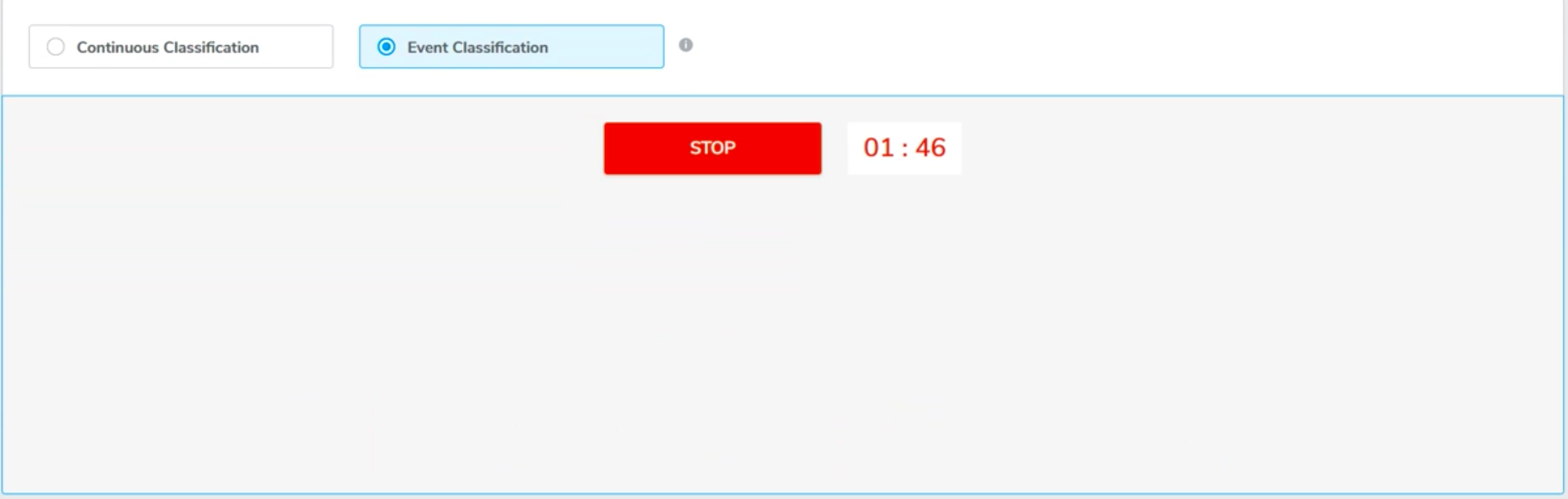
AutoML also supports event classification using hardware button for some target hardware. Press the button on the device to begin the event. The prediction result will display on the screen after the event ends either by releasing the button or the n second of event length is up.
|
|
|
|---|---|---|
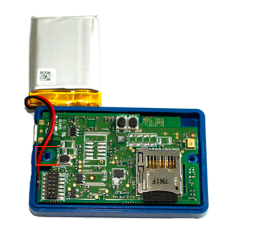 | 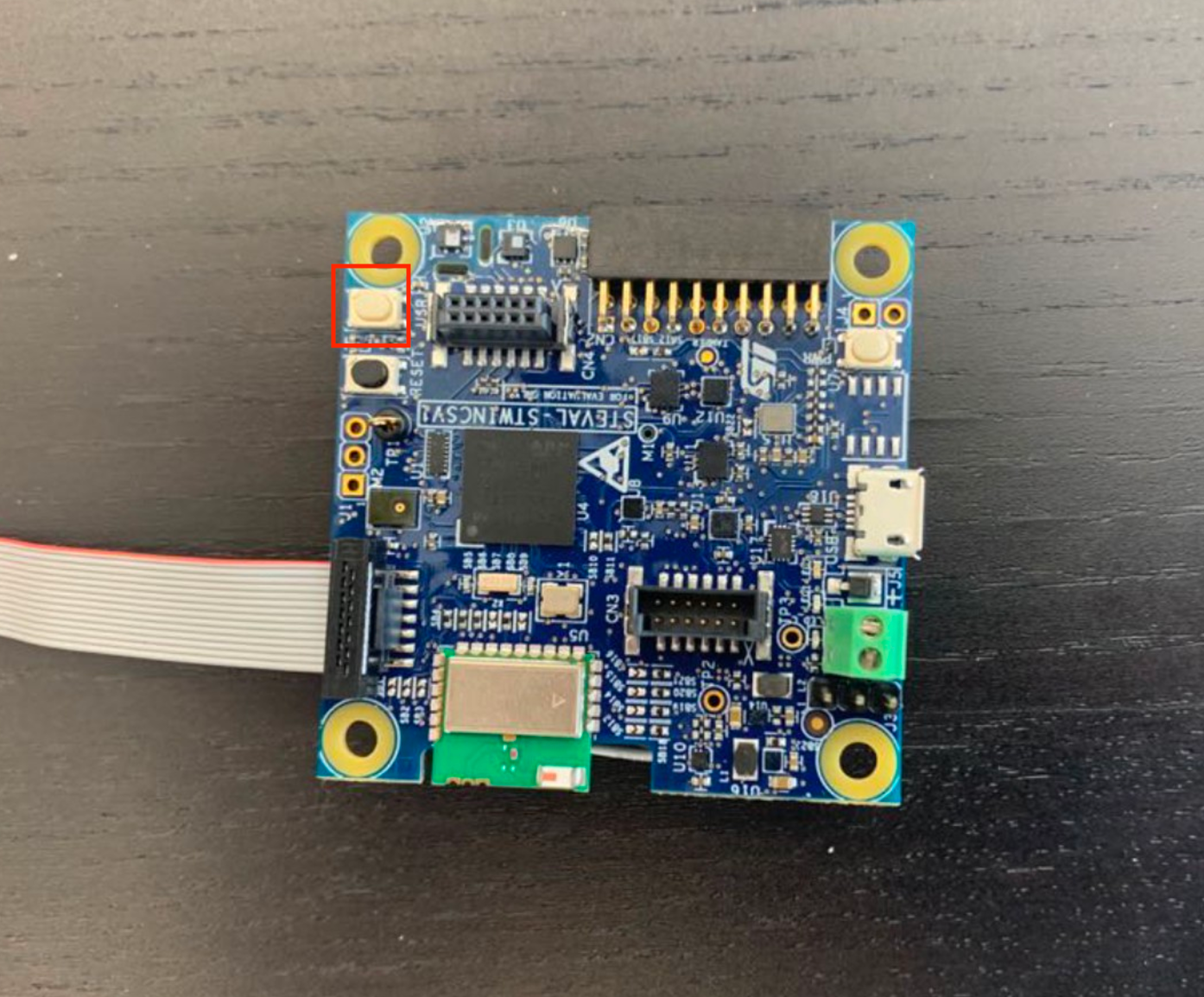 |  |
Contact us and get your own Arduino battery case.
Connection Methods
Click the SELECT CONNECTION METHOD, You can choose between USB and Bluetooth for your device connection.
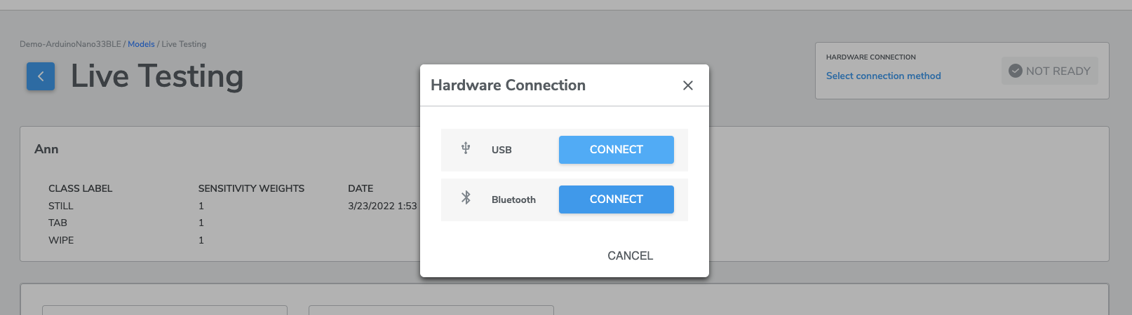
(1) When you press CONNECT for Bluetooth, a screen similar to the following will be presented:
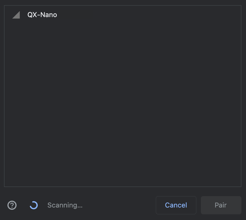
There may be more than one device ready to connect. If so, please choose the one starting with "QX - Nano" to pair with your device.
(2) When you press CONNECT for USB, Live Testing will be conducted via the connected USB cable and no further connection action is required.
For Single-class classification, USB is the only connection method. This is due to limitations for the Manual Calibration option (described below).
Reading Inference from Hardware
We are going to discuss this section with respect to different type of classification type - Multi-class Classification Project, Single-class Classification Project and Multi-Class Anomaly Classification.
(1) Multi-class Classification Project
The machine learning model during live classification outputs two pieces of information: the current predicted class label and the current model output values (called "Probability" in the web app) for each class.
The current predicted class label is based on the class with the highest model output value. Some weighting may also be applied for certain problems, so there may appear to be a minor delay between the maximum class "Probability" and the predicted class label.
The probability table of all class labels are presented as reference.
(2) Single-class Classification Project
For single-class classification, the machine learning model outputs the same two pieces of information. In this case, there will always only be two classes displayed: the given class and the anomaly (i.e. "NON_*") class.
After your single-class model is trained, it may be beneficial to calibrate the threshold of your model to tailor-fit your use case and application scenario. Begin the calibration process by clicking "MANUAL CALIBRATION".
Scores for single-class classifiers are in the range (0, 1], i.e., 0 < Score <= 1. Whether the given instance belongs to the given class or the anomaly class is determined by thresholding the Score, as shown below:
if Score < threshold:
    Signal is Normal
else:
    Signal is Abnormal (i.e. Anomaly)
In the Manual Calibration menu, you can see scores (the blue line) generated by the single-class model plotted over time. Qeexo AutoML recommends an initial threshold based on an analysis of the training data, which is shown by the dotted red line. Users can change the threshold and flash the new, manually-selected threshold to the embedded target. The most recent user-selected threshold is shown in the plot by the dotted green line.
General rules of thumb for threshold tuning is the following:
If you want to be very sensitive to potential anomalies, you should set the threshold to be lower. That means that even small variations in the sensor data away from the collected operating condition would trigger an anomaly. However, please beware that setting the threshold too close to zero may result in too many false positives.
Likewise, if you only want to detect obviously anomalous data, you should keep the threshold to be higher. That means that minor variations in the sensor data away from the collected operating condition may not trigger anomalies.
Please find right balance by doing live classification experiments through live classification after flashing a range of thresholds to the embedded device.
(3) Multi-Class Anomaly Classification
The machine learning model during live classification outputs two pieces of information: the current predicted class label and the current model output values (called "Prediction" in the web app) for each class or the unknown class (If the new datapoint is sufficiently different from any of the training classes). The current predicted class label is based on the class with the highest model output value. In other word, the output can be any of the classes you previously collected just like the Multi-Class classification AND the anomaly (Unknown) class.
The probability table of all class labels are presented as reference
Test Replay (Asynchronous Live Testing)
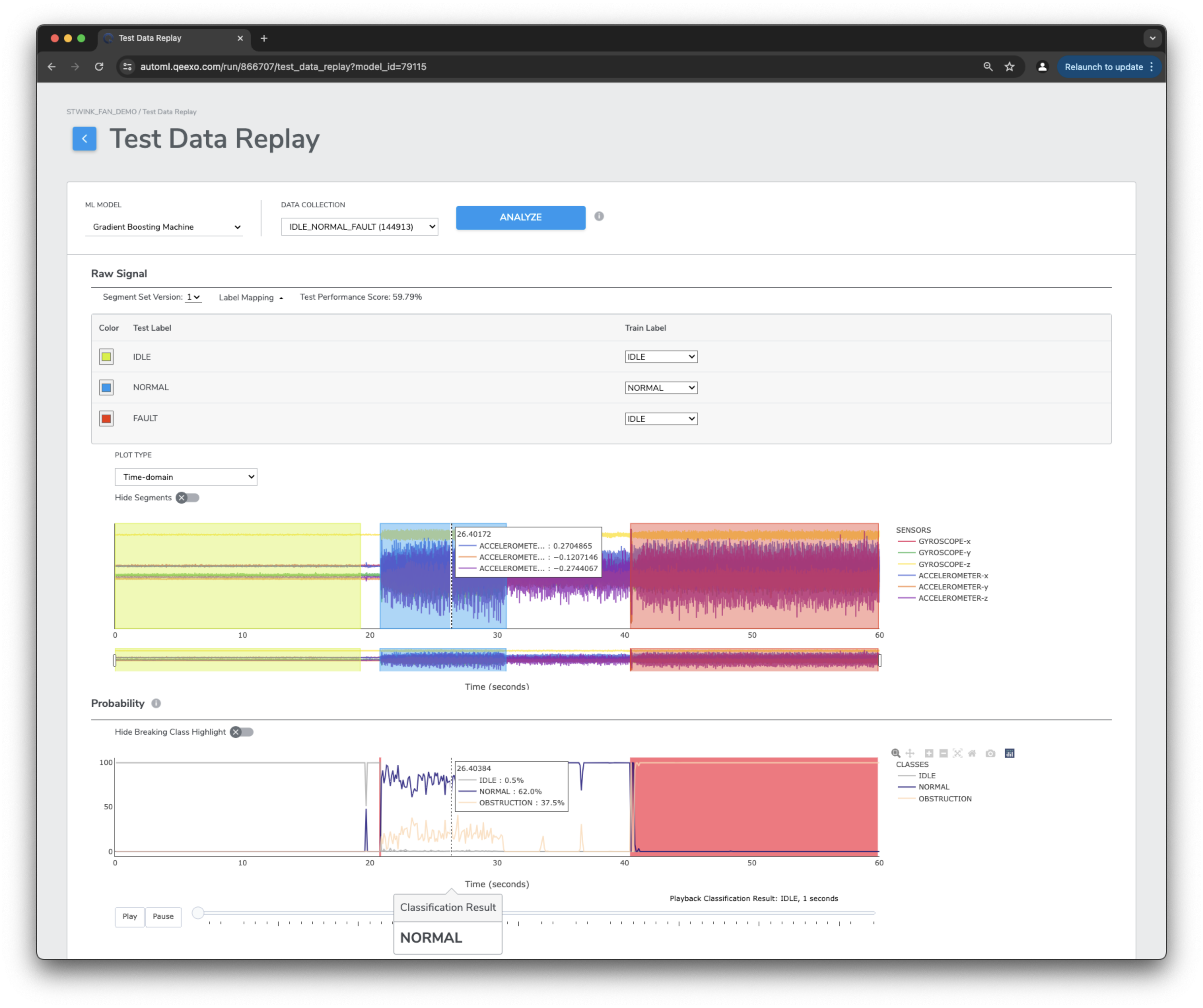
Live Replay provides users with accurate asynchronous live testing capabilities, even without hardware. From the models grid select Live Replay, then choose your test data from the drop dop-down and click Analyze. Behind the scenes Qeexo AutoML will feed your data bit-by-bit into your model and produce inference results that can be replayed at any time. Test replay will also provide you with insights into breaking classes when labeled data doesn’t perform as expected.